Simple steps are all you need

TL;DR: This is an informal summary of our recent paper, to appear in NeurIPS’21, Simple steps are all you need: Frank-Wolfe and generalized self-concordant functions by Alejandro Carderera, Mathieu Besançon, and Sebastian Pokutta, where we present a monotonous version of the Frank-Wolfe algorithm, which together with the simple step size $\gamma_t = 2/(2+t)$ achieves a $\mathcal{O}\left( 1/t \right)$ convergence in primal gap and Frank-Wolfe gap when minimizing Generalized Self-Concordant (GSC) functions over compact convex sets.

Written by Alejandro Carderera.

What is the paper about and why you might care

Consider a problem of the sort: \(\tag{minProblem} \begin{align} \label{eq:minimizationProblem} \min\limits_{x \in \mathcal{X}} f(x), \end{align}\) where $\mathcal{X}$ is a compact convex set and $f(x)$ is a generalized self-concordant (GSC) function. This class of functions, which can informally be defined as those whose third derivative is bounded by their second derivative, have played an important role in the development of polynomial time algorithms for optimization, and also happen to appear in many machine learning problems. For example, the objective function encountered in logistic regression, or in marginal inference with concave maximization [KLS], belong to this family of functions.

As in previous posts, our focus is on Frank-Wolfe or Conditional Gradient algorithms, and we assume that solving an LP over $\mathcal{X}$ is easy, but projecting onto $\mathcal{X}$ is hard, additionally, we assume access to first-order and zeroth-order information about the function. Existing algorithms for this class of functions require access to second-order information, or local smoothness estimates, to achieve a $\mathcal{O}\left( 1/t \right)$ rate of convergence in primal gap [DSSS]. With the Monotonous Frank-Wolfe (M-FW) algorithm we require neither of these, achieving a $\mathcal{O}\left( 1/t \right)$ rate both in primal gap and Frank-Wolfe gap with a simple six-line algorithm that only requires access to a domain oracle, which is simply an oracle that checks if $x \in \mathrm{dom} f$. This extra oracle has to be used if one is to avoid assuming access to second-order information, and is also implicitly used by the existing algorithms that compute local estimates of the smoothness. The proof of convergence for both primal gap and Frank-Wolfe gap are simple and easy to follow, which add to the appeal of the algorithm.

Additionally, we also show improved rates of convergence with a backtracking line search [PNAM] (that locally estimates the smoothness) when the optimum is contained in the interior of $\mathcal{X} \cap \mathrm{dom} f$, when $\mathcal{X}$ is uniformly convex or when $\mathcal{X}$ is a polytope. The contributions are summarized in the table below.

The Monotonous Frank-Wolfe (M-FW) algorithm

Many convergence proofs in optimization make use of the smoothness inequality to bound the progress that an algorithm makes per iteration when moving from $x_{t}$ to $x_{t} + \gamma_t (v_{t} - x_{t})$. For smooth functions this inequality holds globally for all $x_{t}$ and $x_{t} + \gamma_t (v_{t} - x_{t})$. For GSC functions we also have a smoothness-like inequality with which we can bound progress. The problem is that this inequality only holds locally around $x_t$, and if one wants to test if the smoothness-like inequality is valid between $x_t$ and $x_{t} + \gamma_t (v_{t} - x_{t})$ we need to have knowledge of $\nabla^2 f(x_t)$, and know several parameters of the function. Several of the algorithms presented in [DSSS] utilize this approach, in order to compute a step size $\gamma_t$ such that the smoothness-like inequality holds between $x_t$ and $x_{t} + \gamma_t (v_{t} - x_{t})$. Alternatively, one can use the backtracking line search of [PNAM] to find a $\gamma_t$ and a smoothness estimate such that a local smoothness inequality holds between $x_t$ and $x_{t} + \gamma_t (v_{t} - x_{t})$.

We take a different approach to prove a convergence bound, which we review after describing our algorithm. The Monotonous Frank-Wolfe (M-FW) algorithm below is a rather simple, but powerful modification of the standard Frank-Wolfe algorithm, with the only difference that before taking a step, we verify if $x_t +\gamma_t \left( v_t - x_t\right) \in \mathrm{dom} f$, and if so, we check whether moving to the next iterate provides primal progress. Note, that the open-loop step size rule $2/(2+t)$ does not guarantee monotonous primal progress for the vanilla Frank-Wolfe algorithm in general. If either of these two checks fails, we simply do not move: the algorithm sets $x_t = x_{t+1}$. Note that if this is the case we do not need to compute a gradient or an LP call at iteration $t+1$, as we can simply reuse $v_t$.

Monotonous Frank-Wolfe (M-FW) algorithm
Input: Initial point $x_0 \in \mathcal{X}$
Output: Point $x_{T+1} \in \mathcal{X}$
For $t = 1, \dots, T$ do:
\(\quad v_t \leftarrow \mathrm{argmin}_{v \in \mathcal{X}}\left\langle \nabla f(x_t),v \right\rangle\)
\(\quad \gamma_t \leftarrow 2/(2+t)\)
\(\quad x_{t+1} \leftarrow x_t +\gamma_t \left( v_t - x_t\right)\)
\(\quad \text{if } x_{t+1} \notin \mathrm{dom} f \text{ or } f(x_{t+1}) > f(x_t) \text{ then}\)
\(\quad \quad x_{t + 1} \leftarrow x_t\)
End For

The simple structure of the algorithm above allows us to prove a $\mathcal{O}(1/t)$ convergence bound in primal gap and Frank-Wolfe gap. To do this we use an inequality that holds if $d(x_t +\gamma_t \left( v_t - x_t\right), x_t) \leq 1/2$, where $d(x,y)$ is a distance function that depends on the structure of the GSC function. Namely the inequality that we use is: \(\begin{align} f(x_t +\gamma_t \left( v_t - x_t\right)) - f(x^*) \leq (f(x_t)-f(x^*))(1-\gamma_t) + \gamma_t L_{f,x_0}D^2 \omega(1/2), \end{align}\) where $D$ is the diameter of $\mathcal{X}$, and $L_{f,x_0}$ and $\omega(1/2)$ are constants that depend on the function, and the starting point (which we do not need to know). If we were to have knowledge of $\nabla^2 f(x_t)$ we could compute the value of $\gamma_t$ that allows us to ensure that $d(x_t +\gamma_t \left( v_t - x_t\right), x_t) \leq 1/2$, however we purposefully do not want to use second order information!

We briefly (and informally) describe how we prove this convergence bound for the primal gap: As the iterates make monotonous progress, and the step size $\gamma_t = 2/(2+t)$ in our scheme decreases continously, there is an iteration $T$, which depends on the function, after which the smoothness-like inequality holds for all $t \geq T$ between $x_t$ and $x_t +\gamma_t \left( v_t - x_t\right)\in \mathrm{dom} f$, i.e. we guarantee that $d(x_t +\gamma_t \left( v_t - x_t\right), x_t) \leq 1/2$ for $t \geq T$ (without the need to know any parameters). However, note that in order to take a non-zero step size we also need to ensure that $f(x_{t+1}) < f(x_t)$. We complete the convergence proof using induction, that is, the assumption that $f(x_t) - f(x^\esx) \leq C(T+1)/(t+1)$ where $C$ is a constant, and the following subtlety – the smoothness-like inequality will only guarantee progress (i.e. $f(x_{t+1}) < f(x_t)$) at iteration $t$ if $\gamma_t$ is smaller than the primal gap at iteration $t$ multiplied by a factor. We can see this by going to the inequality above, and seeing that we will be able to guarantee that $f(x_{t+1}) < f(x_t)$ if: \(\begin{align} \gamma_t(f(x_t) - f(x^*)) - \gamma_t^2L_{f,x_0}D^2 \omega(1/2) <0, \end{align}\) If this is true, we can guarantee that we set $x_{t+1} = x_t +\gamma_t \left( v_t - x_t\right)$ and we can bound the progress using the smoothness-like inequality. Using the aforementioned fact and our induction hypothesis that \(f(x_t) - f(x^\esx) \leq C(T+1)/(t+1)\), we prove that claim $f(x_{t+1}) - f(x^\esx) \leq C(T+1)/(t+2)$. Assume however that this is not the case and that the following inequality is true: \(\begin{align} \gamma_t(f(x_t) - f(x^*)) - \gamma_t^2L_{f,x_0}D^2 \omega(1/2) \geq 0. \end{align}\) Reordering the previous expression, we have that $f(x_t) - f(x^*) \leq \gamma_t L_{f,x_0}D^2 \omega(1/2)$, with $\gamma_t = 2/(2+t)$. It turns out that $\gamma_t L_{f,x_0}D^2 \omega(1/2) \leq C(T+1)/(t+2)$, so there is nothing left to prove, and we do not even need the induction hypothesis, as for this case the claim is automatically true for $t+1$. The proof of convergence in Frank-Wolfe gap proceeds similarly. See Theorem 2.5 and Theorem A.2 in the paper for the full details.

Complexity Analysis

As each iteration of the algorithm computes at most one first-order oracle call, one zeroth-order oracle call, one LP call, and one domain oracle call, we can bound the number of oracle calls needed to achieve an $\epsilon$ tolerance in primal gap (or Frank-Wolfe gap) directly using the iteration-complexity bound of $\mathcal{O}(1/\epsilon)$.

Note also that we can also implement the M-FW algorithm using a halving strategy for the step size, instead of the $2/(2+t)$ step size. This strategy helps deal with the case in which a large number of consecutive step sizes $\gamma_t$ are rejected either because $x_t + \gamma_t(v_t - x_t) \notin \mathrm{dom} f$ or $f(x_t) < f(x_t + \gamma_t(v_t - x_t))$. The strategy consists of halving the step size if we encounter any of these two cases. This results in a step size that is at most a factor of 2 smaller than the one that would have been accepted with the original strategy. However, the number of zeroth-order or domain oracles that would be needed to find this step size that satisfies the desired properties is logarithmic when compared to the number needed for the $2/(2+t)$ variant. The convergence properties established throughout the paper for the M-FW also hold for the variant with the halving strategy; with the only difference being that we lose a small constant factor in the convergence rate.

Computational Experiments

We compare the performance of the M-FW algorithm with that of other projection free algorithms which apply to the GSC setting. That is, we compare to the B-FW and the GSC-FW algorithms of [DSSS], the non-monotonous standard FW algorithm, for which there are no formal convergence guarantees for this class of problems, and the B-AFW algorithm. Note that the B-AFW is simply the AFW algorithm with the backtracking strategy of [PNAM], for which we also provide convergence guarantees in some special cases in the paper for GSC functions.

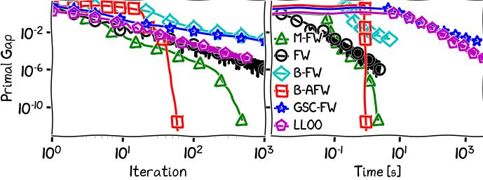
Figure 1. Portfolio Optimization.

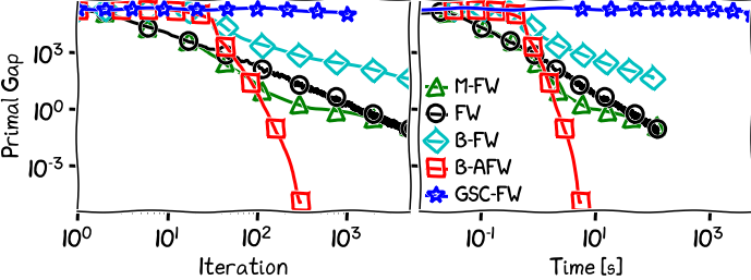
Figure 2. Signal recovery with KL divergence.

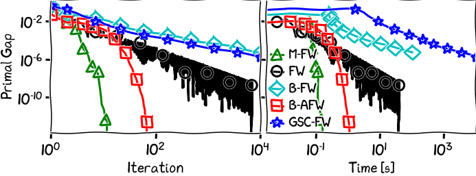
Figure 3. Logistic regression over $\ell_1$ unit ball.

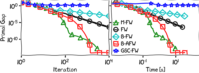
Figure 4. Logistic regression over the Birkhoff polytope.

References

[KLS] Krishnan, R. G., Lacoste-Julien, S., and Sontag, D. Barrier Frank-Wolfe for Marginal Inference. In Proceedings of the 28th Conference in Neural Information Processing Systems. PMLR, 2015. pdf

[DSSS] Dvurechensky, P., Safin, K., Shtern, S., and Staudigl, M. Generalized self-concordant analysis of Frank-Wolfe algorithms. arXiv preprint arXiv:2010.01009, 2020b. pdf

[PNAM] Pedregosa, F., & Negiar, G. & Askari, A. & Jaggi, M. (2020). Linearly Convergent Frank-Wolfe with Backtracking Line-Search. In Proceedings of the 23rd International Conference on Artificial Intelligence and Statistics. pdf