Emulating the Expert
TL;DR: This is an informal summary of our recent paper An Online-Learning Approach to Inverse Optimization with Andreas Bärmann, Alexander Martin, and Oskar Schneider, where we show how methods from online learning can be used to learn a hidden objective of a decision-maker in the context of Mixed-Integer Programs and more general (not necessarily convex) optimization problems.
What is the paper about and why you might care
We often face the situation in which we observe a decision-maker—let’s call her Alice—who is making “reasonably optimal” decisions with respect to some private objective function and another party—let’s call him Bob—would like to make decisions that emulate Alice’s decisions in terms of quality with respect to Alice’s private objective function. Classical applications where this naturally occurs is in the context of learning customer preferences from observed behavior in order to recommend new products etc. that match the customer’s preference or for example in dynamic routing, where we observe routing decisions of individual participants but we cannot directly observe, e.g., travel times. The formal name for the problem that we consider is inverse optimization; informally speaking we can say we simply want to emulate the expert. For completeness, in reinforcement learning we would refer to what we want to achieve as inverse reinforcement learning.
The following graph lays out the basic setup that we consider:
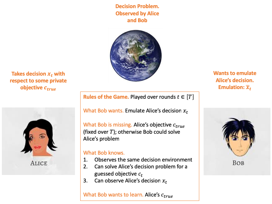
In summary, Alice is solving
\[x_t \doteq \arg \min_{x \in P_t} c_{true}^\intercal x,\]and Bob can solve
\[\bar x_t \doteq \arg \min_{x \in P_t} c_t^\intercal x,\]for some guessed objective $c_t$ and after Bob played his decision $\bar x_t$, he observes Alice decision $x_t$ taken with respect to her private objective $c_{true}$. For each time step $t \in [T]$, the $P_t$ is some feasible set of decisions over which Alice and Bob can optimize their respective (linear) objective functions; the interesting case is where $P_t$ varies over time, so that Alice’s decision $x_t$ is round-dependent. Note, that we can basically accommodate arbitrary (potentially non-linear) function families as long as we have a reasonable “basis” for this family; the interested reader might check the paper for details.
Learning to emulate Alice’s decisions $x_t$ seems to be almost impossible to accomplish at first:
- We obtain potentially very little information only from Alice’s decision $x_t$.
- The objective that explains Alice’s decisions might not be unique.
However, it turns out that under reasonable assumptions, such that Alice’s decisions are reasonably close to the optimal ones with respect to $c_{true}$ and with an amount of examples that are “diverse enough” as necessitated by the specifics of the instance, we in fact can learn an equivalent objective that renders Alice’s solutions basically optimal w.r.t. this learned proxy objective. In fact, one way to solve an offline variant of this problem to obtain such a proxy objective that is quite well known is via dualization or KKT system approaches. For example in the case of linear programs this can be done as follows:
Remark (LP case). Suppose that $P_t \doteq \setb{x \in \RR^n \mid A_t x \leq b_t}$ for $ t \in [T]$ and assume that we have a polyhedral feasible region $F = \setb{c \in \RR^n \mid Bc \leq d}$ for the candidate objectives. Then the linear program \[ \min \sum_{t = 1}^T (b_t^\intercal y_t - c^\intercal x_t) \qquad \] \[ A_t^\intercal y_t = c \qquad \forall t \in [T] \] \[ y_t \geq 0 \qquad \forall t \in [T] \] \[ Bc \leq d, \] where $c$ and the $y_t$ are variables and the rest is input data, computes a linear objective $c$, if feasible and bounded etc, so that for all $t \in [T]$ it holds \[ c^\intercal x_t = \max_{x \in P} c_{true}^\intercal x. \]
While the above can also be reasonably extended to convex programs via solving the KKT system instead, it has two disadvantages:
- It is an offline approach: first collect data and then regress out a proxy objective, i.e., first-learn-then-optimize, which might be problematic in many applications.
- Additionally, and not less severe, this only works for linear programs (convex programs) and not Mixed-Integer Programs or more general optimization problems as, due to non-convexity, the KKT system or the dual program is not defined/available in this case.
Our results
Our method alleviates both of the above shortcomings, by providing an online learning algorithm, where we learn a proxy objective equivalent to Alice’s objective while we are participating in the decision-making process, i.e., our algorithm is an online algorithm. Moreover, our approach is general enough to apply to a wide variety of optimization problems (including MIPs etc) as it only relies on standard regret guarantees and (approximate) optimality of Alice’s decisions. More precisely, we provide an online learning algorithm—using either Multiplicative Weights Updates (MWU) or Online Gradient Descent (OGD) as a black box—that ensures the following guarantee.
Theorem [BMPS, BPS]. With the notation from above the online learning algorithm ensures \[ 0 \leq \frac{1}{T} \sum_{t = 1}^T (c_t - c_{true})^\intercal (\bar x_t - x_t) \leq O\left(\sqrt{\frac{1}{T}}\right), \] where the constant hidden in the $O$-notation depends on the used algorithm (either MWU or OGD) and the (maximum) diameter of the feasible regions $P_t$.
In particular, note that in the above
\[(c_t - c_{true})^\intercal (\bar x_t - x_t) = \underbrace{c_t^\intercal (\bar x_t - x_t)}_{\geq 0} + \underbrace{c_{true}^\intercal (x_t - \bar x_t)}_{\geq 0},\]where the nonnegativity arises from the optimality of $x_t$ w.r.t. $c_{true}$ and the optimality of $\bar x_t$ w.r.t. $c_t$. We therefore obtain in particular that
\[ 0 \leq \frac{1}{T} \sum_{t = 1}^T c_t^\intercal (\bar x_t - x_t) \leq O\left(\sqrt{\frac{1}{T}}\right), \]
and
\[ 0 \leq \frac{1}{T} \sum_{t = 1}^T c_{true}^\intercal (x_t - \bar x_t) \leq O\left(\sqrt{\frac{1}{T}}\right), \]
hold, which tend to $0$ on the right-hand side for $T \rightarrow \infty$. Thus Bob’s decisions $\bar x_t$ converge to decisions that are not only close in cost, on average, compared to Alice’s decisions $x_t$ w.r.t. to $c_t$ but also w.r.t. to $c_{true}$ although we might never actually observe $c_{true}$. In the paper we consider also special cases under which we can ensure to recover $c_{true}$ and not just an equivalent function. One way of thinking about our online learning algorithm is that it provides an approximate solution to the (inaccessible) KKT system that we would like to solve. In fact in the case of, e.g., LPs it can be shown that our algorithm solves a dual program similar to the one from above by means of gradient descent (or mirror descent).
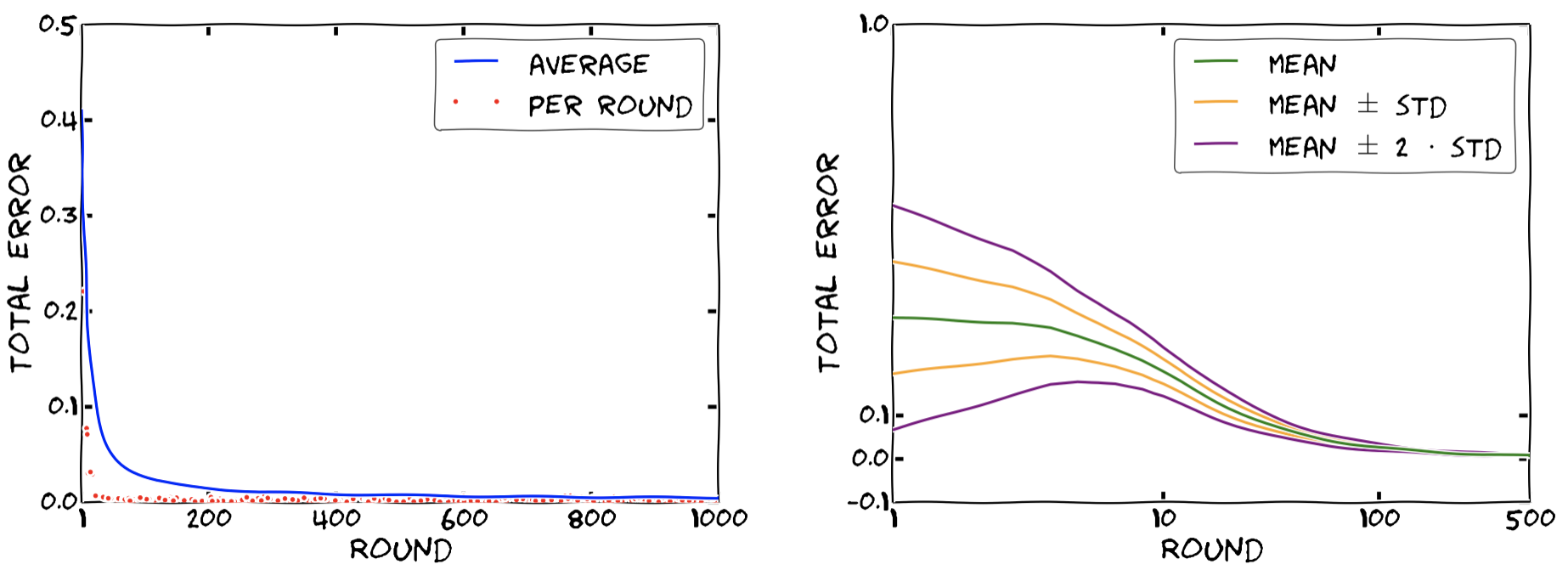
The key question of course is, whether our algorithm actually also works in practice. And the answer is yes. The left plot shows the convergence of the total error $(c_t - c_{true})^\intercal (\bar x_t - x_t)$ over $t \in [T]$ in each round (red dots) as well as the cumulative average error up to that point (blue line) for an integer knapsack problem with $n = 1000$ items over $T = 1000$ rounds using MWU as black box algorithm. The proposed algorithm is also rather stable and consistent across instances in terms of convergence, as can be seen in the right plot, where we consider the statistics of the total error over $500$ runs for a linear knapsack problem with $n = 50$ items over $T = 500$ rounds. Here we depict mean total error averaged up to that point in time $\ell$, i.e., $\frac{1}{\ell} \sum_{t = 1}^{\ell} (c_t - c_{true})^\intercal (\bar x_t - x_t)$ and associated error bands.
A note on generalization
If the varying decision environments $P_t$ are drawn i.i.d. from some distribution $\mathcal D$, then also a reasonable form of generalization to unseen realizations of the decision environment $P_t$ drawn from distribution $\mathcal D$ can be shown, provided that we have seen enough examples within the learning process. For this one can show that after a sufficient number of samples $T$ it holds
\[ \frac{1}{T} \sum_{t = 1}^T c_{true}^\intercal x_t \approx \mathbb E_{\mathcal D} [c_{true}^\intercal \tilde x], \]
where $\tilde x = \arg \max_{x \in P} c_{true}^\intercal x$ for $P \sim \mathcal D$ and one then applies the regret bound, which provides
\[ \frac{1}{T} \sum_{t = 1}^T c_{true}^\intercal x_t \approx \frac{1}{T} \sum_{t = 1}^T c_{true}^\intercal \bar x_t, \]
so that roughly
\[ \frac{1}{T} \sum_{t = 1}^T c_{true}^\intercal \bar x_t \approx \mathbb E_{\mathcal D} [c_{true}^\intercal \tilde x] , \]
follows. This can be made precise by working out the number of samples, so that the approximation errors above are of the order of a given $\varepsilon > 0$.
References
[BMPS] Bärmann, A., Martin, A., Pokutta, S., & Schneider, O. (2018). An Online-Learning Approach to Inverse Optimization. arXiv preprint arXiv:1810.12997. arxiv
[BPS] Bärmann, A., Pokutta, S., & Schneider, O. (2017, July). Emulating the Expert: Inverse Optimization through Online Learning. In International Conference on Machine Learning (pp. 400-410). pdf
Comments