H-index and Citations
TL;DR: Total cites vs. H-index and some numbers.
In this very compact blog post, I want to briefly summarize the dynamics between total citations and the h-index, a crucial metric in academia. Essentially, this discussion revolves around the total citations of a researcher and how these citations can be partitioned into integer partitions. The h-index is then closely connected to Durfee squares of these integer partitions.
Understanding the H-index
The h-index, proposed by Jorge Hirsch in 2005, is a metric that aims to measure both the productivity and citation impact of the publications of a researcher. Specifically, a scientist has an index of $h$ if $h$ of their $N_p$ papers have at least $h$ citations each, and the other $N_p - h$ papers have no more than $h$ citations each. This index helps to gauge the cumulative impact of a researcher’s work without being overly influenced by a small number of highly cited papers or by many papers with few citations.
An Important Formula
One useful approximation for estimating the h-index is given by Hirsch (2005) and is particularly valuable for understanding the relationship between the h-index and total citations. The approximation is:
\[\tag{estimation} h \approx \alpha \sqrt{c},\]where $\alpha \in [0.45,0.58]$ (Hirsch used $0.54$ himself). This formula can also be expressed as $h \approx \sqrt{c/\beta}$ with $\beta \in [3,5]$, leading to $\alpha = \sqrt{1/\beta}$. Equivalently, the relationship can be reversed to estimate the total citations from the h-index:
\[c \approx \left(\frac{h}{\alpha}\right)^2.\]Example Calculation
To illustrate, let us use the upper bound of $\alpha$ as $0.54$, as suggested by Hirsch. An h-index of $30$ corresponds then to citations in the range $[3086, 4444]$. Conversely, 3000 citations would correspond to an h-index range of $[24.6, 29.6]$, which rounds to $[25, 30]$. It is noteworthy that in the h-to-c direction, the sensitivity is somewhat high, i.e., an estimation error of a factor of $2$ in $h$ translates to an error of a factor of $4$ in $c$, while the other direction is much more stable: a factor of $2$ in estimating citations leads to only a factor of $\sqrt{2} \approx 1.41$ in error, i.e., about $41\%$.
Upper and Lower Bounds
Using the estimation formula, we can now compare total citations against upper and lower citation bands induced by the h-index and vice versa. The following graphic illustrates this comparison based on data (total citations and h-index at that time) from 15 researchers.
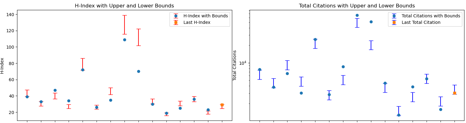
Figure 1. Left: h-index and bands implied by total citations. Right: total citations and bands implied by h-index; the right scale is log-scale. The last data point being the weighted aggregate for the cohort.
Fitting a Quadratic
For a more precise calibration tailored to an individual researcher, one can (linearly) fit the h-index against the square root of their total citations over time. This method might provide a more stable estimate than using the general rule-of-thumb mentioned earlier and gives the relationship:
\[h = \alpha \sqrt{c} + \beta,\]where $\alpha, \beta$ are the coefficients obtained from the linear regression.
Dynamics of the h-index
Under reasonable assumptions the h-index grows linearly in time. There are basically two arguments to it. First, it is proportional to the square root of citations that grow quadratically (up to a certain point). Second, we can use a simple model. Suppose publications are arriving at a rate $\alpha$ and then accumulate citations at a rate $\beta$. Then in order get an h-index of $k$ the $k$-th publication has to arrive and then produce $k$ citations, i.e., it takes time:
\[k (\alpha + \beta),\]and hence is linear in $k$.
Some properties about exponential growth
We will now briefly discuss the dynamics of exponential growth and in particular the growth rate of total citations vs. the growth rate of citations in a given year. Note that we assume geometric growth here which might be unrealistics in the long-run but ok for shorter time intervals.
We consider two models: the continuous discounting model and the discrete discounting model.
| continuous discounting | discrete discounting | |
|---|---|---|
| total citations: \(f(t)\) | \(e^{rt}\) | \((1+r)^t\) |
| citations in year \(t\): \(f'(t)\) | \(r e^{rt}\) | \(r (1+r)^{t}\) |
Note that in the above for the continuous case we indeed have the derivative but for the discrete case, this is slightly different with \(r (1+r)^{t}\) being the new citations in the year \(t+1\); this is not the derivative but basically the integral of derivative over the year. Here we account for the new citations upcoming in the year \(t+1\) computed at the end of the year \(t\), i.e., \((1+r)^t\) is the total citations at the end of year \(t\) and then we have a growth of \(r\) in the next year. If we would do it the other way around, i.e., the new citations for year \(t\), then the formula would be \(r (1+r)^{t-1}\) and the changes would propagate accordingly.
Discrete discounting. For the function $f(t) = (1+r)^t$ we have:
\[\frac{(1+r)^{t+1}}{(1+r)^t} = 1+r\]and for the derivative we have:
\[\frac{(1+r)^{t+1}r}{(1+r)^{t}r} = 1+r,\]hence the growth rate of the total citations and the growth rate of the citations in a given year are the same.
Continuous discounting. For the function $f(t) = e^{rt}$ we have:
\[\frac{e^{r(t+1)}}{e^{rt}} = e^r,\]and for the derivative we have:
\[\frac{e^{r(t+1)}r}{e^{rt}r} = e^r,\]hence the growth rate of the total citations and the growth rate of the citations in a given year are the same.
Offset between total citations and citations in a given year. This basically captures hold long it takes in years until the new citations per year become the total citations.
For the continuous case we have:
\[e^{rt} = r e^{r(t+\Delta)} \Leftrightarrow 1 = r e^{r\Delta} \Leftrightarrow \Delta = \frac{\ln(1/r)}{r}.\]For the discrete case we have:
\[(1+r)^t = r (1+r)^{t+\Delta} \Leftrightarrow 1 = r (1+r)^{\Delta} \Leftrightarrow \Delta = \frac{\ln(1/r)}{\ln(1+r)}.\]As we can see, the offset is slightly larger for the discrete case. This is due to accounting differences as in the discrete case we “observe” the new citations only at the end of the year. Also note that we do not use the approximation \(\ln(1+r) \approx r\) as $r$ might be quite large, so that the approximation is not good.
| r | continuous offset | discrete offset |
|---|---|---|
| 0.05 | 59.91 | 61.40 |
| 0.1 | 23.03 | 24.16 |
| 0.2 | 8.05 | 8.83 |
| 0.3 | 4.01 | 4.59 |
| 0.4 | 2.29 | 2.72 |
Skewed H-indices: Beyond the Durfee Square
While the standard H-index measures the size of the largest square that fits under the citation curve (the Durfee square), one can refine this picture by “skewing” the square into a rectangle. Two natural variants are:
-
High-impact core (\(h_2\)):
\[h_{2} = \max\bigl\{\,h : \text{the $h$-th paper has at least $2h$ citations}\bigr\}.\]In Durfee-language, this is the side-length of the largest \(h\times2h\) rectangle under the Ferrers diagram. By focusing on papers cited twice as often as their rank, \(h_2\) isolates the very top-tier work. A ratio \(h_2/h\) close to 1 means most of the h-core papers are well above the plain h-bar.
-
Standard H-index (\(h\) or \(h_1\)):
\[h = \max\bigl\{\,h : \text{the $h$-th paper has at least $h$ citations}\bigr\},\]recovering the usual Durfee square.
-
Broad impact tail (\(h_{1/2}\)):
\[h_{1/2} = \max\bigl\{\,h : \text{the $h$-th paper has at least $\tfrac h2$ citations}\bigr\}.\]Here we fit the largest \(h\times\lfloor h/2\rfloor\) rectangle under the diagram, i.e. count how many papers have at least half as many citations as their position. This index captures the depth of the productive tail: a long list of solidly cited papers.
What these variants reveal
-
Monotonicity
\[h_{2} \le h \le h_{1/2}.\]A stricter threshold (2× rank) gives a smaller core; a looser one (½× rank) gives a larger tail.
-
Performance interpretation
- \(h_2\) measures the exceptional works—the number of papers not just above the H-bar but comfortably above it.
- \(h_1\) is the classic balance of quantity and impact.
- \(h_{1/2}\) gauges the breadth of respectable influence—how far the “long tail” of moderately cited papers extends.
Together, (\(h_2\), \(h_1\), \(h_{1/2}\)) sketch the shape of a citation profile: the steepness at the top, the central plateau, and the depth of the tail.
Comments