Demographic Shift: A wave is coming

TL;DR: Basic effects of demographic shifts and some mechanics. Mostly for my own reference.

Disclaimer. This is neither a comprehensive analysis nor a prediction. Rather it is a simple overview and model mostly for my own reference. Read with care and understand the simplifications and assumptions made. Think of it as my private notes.

Introduction

Most developed countries face a significant demographic shift: The population is aging and shrinking, and birth rates are low. This has significant implications for basic economics. The effect is so pronounced that it will be hard, if not impossible, to mitigate it. Moreover, there is a significant delay in the system, so countermeasures will only manifest in the long run (about 30 years from now). While some aspects are specific to Germany, most effects hold more broadly. In particular, the effects are mostly data insensitive as we will see later with only a couple of variables (in particular fertility rates and to some extent mortality rates) really driving the main effects.

In the following we will consider a couple of key points:

Young vs Old: The age-dependency ratio is shifting, with more elderly dependents compared to the working-age population.
Net Giver to Net Taker: Individuals who were net givers in the past become net takers in their old age. Depending on the demographic structure this might induce severe “cash-flow” reversals. Note: (a) we use these terms strictly as technical terms; no judgement etc at any time. (b) the attribution is point-in-time.
Immigration: We do not explicitly consider immigration here as it is a complex topic beyond the scope. Immigration can help mitigate some of the effects but is not a silver bullet. In particular, immigration beyond the reproductive bracket (more on this later) will not impact fertility rates and generally the effects are quantitatively small; see data below.
Generational Contract: In countries like Germany, the generational contract results in high intergenerational dependence. This is slightly different in countries like the US, where intergenerational transfer is less pronounced, and people save for their own retirement. For more Germany-specific details, see the Generationenvertrag Wikipedia page. Here is a summary of the Wikipedia article from the best intern of the relevant points for the discussion at hand:

The demographic shift is putting immense strain on Germany’s social systems, especially the pension system based on the “Generationenvertrag” (generational contract). Currently, a shrinking workforce supports a growing elderly population, with a significant rise in people over 67 and an increasing average age, which reached 45.7 years by 2020. The portion of people over 85 quadrupled from 1970 to 2018, reaching 2.3 million.

From 2025, when Germany’s largest birth cohorts begin retiring, pension funding will face a critical shortfall. If no sustainable solution is implemented, taxes like VAT could need to increase from 19% to 26%. Maintaining current pension levels may require those born in 1985 to work until age 72 to enjoy a retirement period similar to today’s retirees.

Additional concerns include low-wage workers and self-employed individuals, who face a high risk of poverty in old age. The statutory pension system advises supplementary private or corporate pensions to maintain living standards in retirement.

Wait a second, how does VAT and income tax come into the picture? The numbers for Germany are roughly as follows: In 2024, 37.1% of taxes were allocated to social security-like line items (pension, unemployment, etc.). While these line items are not only funded by invidual taxes (there is also corporate tax, tariffs, etc.), about 36.8% of taxes came from income tax and about 28.2% from VAT, totalling about 65% of all taxes; see here for breakdown. These numbers vary year-by-year but not by that much.

Note.

As often the case, while many data sources disagree on the micro level, they tend to agree on the macro level, i.e., different studies find different numbers but the overall picture is the same. Thus, take the exact numbers with a grain of salt.
There is also a point to be made that having children is a vote of confidence in the future and the development of the country of residence; and the lack of children can be seen as an expression of disillusionment. This is somewhat related to the so-called demographic winter; see also here for an overview of South Korea’s situation, currently sporting the lowest fertility rate in the world with $0.72$ children per woman. Interestingly, there is also an inverse correlation between income and fertility rate, see here.
There are also workforce considerations that are closely related to the demographic shift as well as the potential use of AI technologies that might offset some of the adverse effects. However, this is beyond the scope of this note and might be explored in a future note.

Relevant Data

In the following we provide some data relevant for the discussion. Most of it is collected from various sources from the internet and I did some very basic consistency checks only; so beware.

Fertility Rates

The first relevant data point is fertility rates (sometimes also called (total) birth rates; we will use both terms interchangeably here). These rates are a key driver of the demographic shift and have been continuously declining over the past decades in developed countries. The most recent data for Germany from 2023 is around 1.35 births per woman. This is considerably below the replacement rate of roughly 2.1 children per woman, which is the threshold for a stable population. The 2.1 decomposes into 2 for obvious reasons and the (roughly) 0.1 accounts for (infant) mortality and other factors (such as a slighter higher proportion of men born but with a lower life expectancy) reducing the number of women in the relevant age bracket. See also net reproduction rate, that takes these effects into account by measuring the average number of daughters per woman and hence “renormalizes” the fertility rate; we capture the same effects but bake them back into the typically reported (total) fertility rate notion if not stated otherwise.

The figure below shows the fertility rates for various countries up to $2017$; the data is from the World Bank. The trend basically continued for all countries until $2024$ but I could not find publicly available data, consistent across multiple countries until $2024$.

Figure 1. Fertility rates. Source: World Bank

Net Giver vs Net Taker

Another important data point is the distribution between net giver and net taker as function of age. As we can see in the graphics the roles switch around over the years and will become relevant later in the context of age dependency ratios; data is from IW Köln for Germany. The coloring, corresponding to the various types of income/expense streams can be ignored for the discussion at hand; the interested reader is referred to the original source.

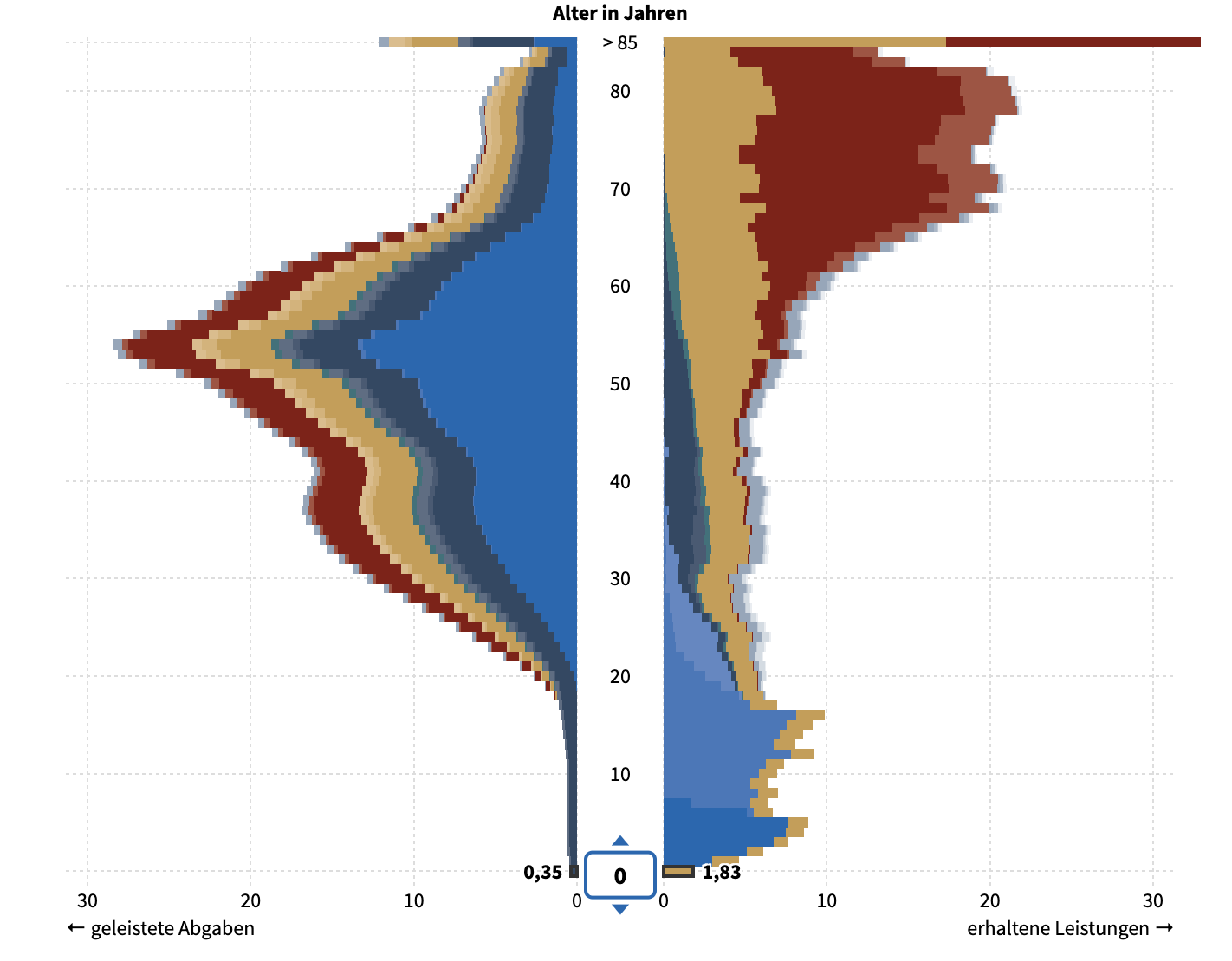
Figure 2. Net giver vs net taker. Source: IW Köln

Projections of demographic development

The following three figures show some projections of the German population. The first figure shows the population aged 67 and over, which will be important when we later consider old-age dependency ratios.

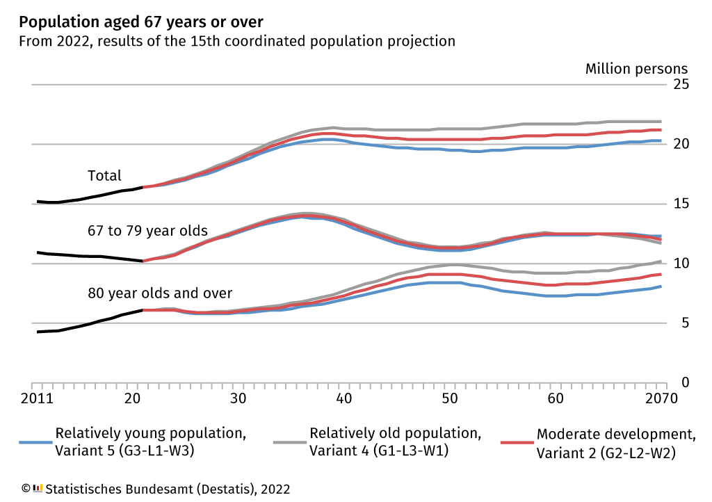
Figure 3. German population aged 67 and over. Source: Statitisches Bundesamt

The second figure shows two different projections of the German population and the impact of immigration on the demographic shift.

Figure 4. Two different projections of the German population. Source: DIW Berlin

The third figure shows the development of the population pyramid of Germany over time. Observe the tapering towards the later years.

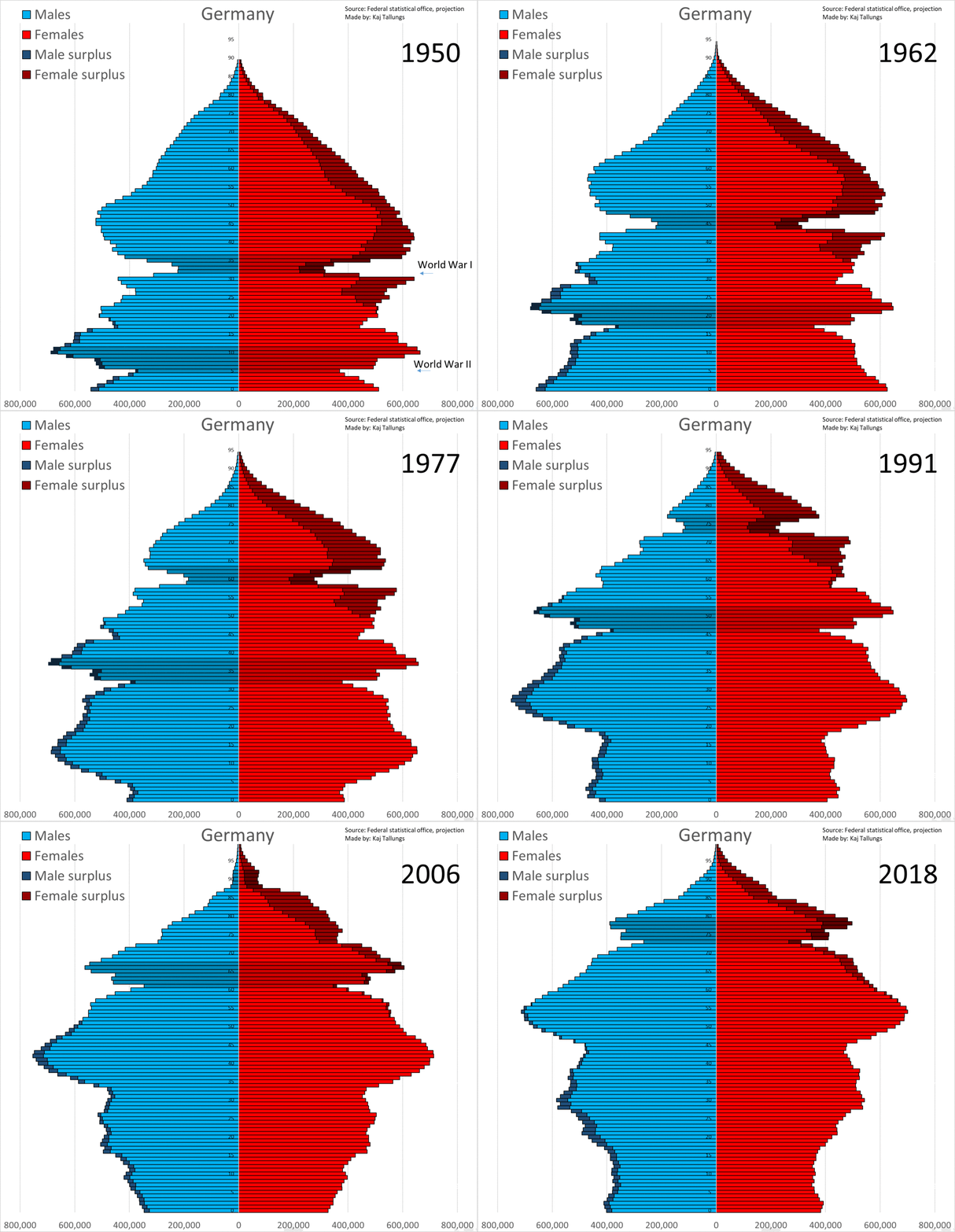
Figure 5. Population pyramid of Germany over time. Source: Wikipedia

While we will not directly work with this data it is instrumental in understanding some of the overall trends.

Age Dependency Ratios

This brings us to the next important data point: age dependency ratios. These ratios capture basically non-working population relative to the working-age population; we will discuss this further below. The following two figures show the age dependency ratio for Germany (and the world) arising from two different data sources and scenarios.

The first figure shows the age dependency ratio for the world and Germany according to the World Bank.

Figure 6. Age dependency ratio for the world and Germany. Source: Google Public Data

The second figure focuses on the (so-called) old-age dependency ratio for Germany according to Eurostat.

Figure 7. Old-age dependency ratio for Germany. Source: Google Public Data

Taxation

As a point of reference we depict the current income tax rates for Germany (2024) in the following table and figure, respectively. These are relevant in terms of the tax revenue discussion from before as well as the old-age dependency ratio further below.

Income over (single)	Income over (married)	Marginal rate range
€0	€0	0%
€11,604	€23,208	14%-24%
€17,005	€34,010	24%-42%
€66,760	€133,520	42%
€277,826	€555,650	45%

The figure below contains also the effective tax rates for various income brackets for single and married individuals.

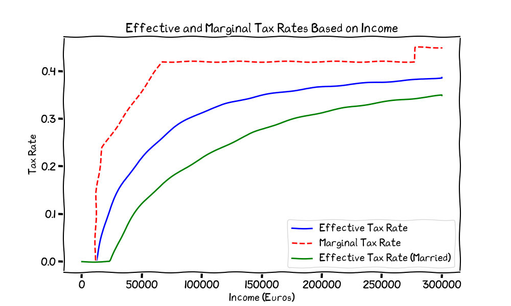
Figure 8. Taxation in Germany.

A simple model

With this out of the way we can now move on to our simple model that we will use; see also the figure below. The simple demographic model is designed to simulate population dynamics by focusing on key age brackets and their roles in shaping the population structure. Births predominantly occur within the 20-29 age bracket, which is crucial for obtaining the next generation that enters the population in the following time step. It is this reproductive bracket that is key for general population growth and demographic tilt; note that we simplify here since the average age of childbearing in Germany is around 30.3 years. However, this is not that important for the overall dynamics and it serves as a compromise between different countries, and places childbearing at the beginning of the working-age bracket; simply “rescaling (or rubberbanding) the grid” allows to generalize to other cases and also note that due to the structure of our model where one time-step is one decade, the next generation comes online around $30$ years later. This last part is particularly important: the cycle of reproduction induces about a 30-year delay until changes in birth rates are reflected in the population pyramid. Beyond the reproductive age bracket, mortality rates become the main influence on the population pyramid, with the most significant impact observed in the older age brackets, particularly those aged 60 and above. The last bracket is the 90+ age bracket, integrating the tail, and is sometimes relatively larger than the bracket before; while an artifact of the simple model this is not an issue. The model advances by decades (i.e., one time step is 10 years) as mentioned before. As a consequence of this simplifcation the model can show pronounced jumps every three decades, i.e., when the offspring from the reproductive age bracket enters the population; this is more of a feature than a bug as it emphasizes the impact of fertility rates and its delay.

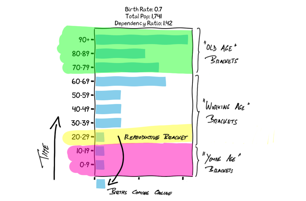
Figure 9. Basic structure of demographic model.

Now let us look at some very basic consequences first.

Replacement rate. First, there exist a rate $r_0$, the so-called replacement rate, so that size of the reproductive age bracket is stable over time. For Germany this rate is about $2.1$ children per woman; see above when where discussed fertility rates. In our simplified model it is roughly $2.02$ as we ignore differences in male vs female offspring for example (and some other factors); the effect is minor.

Fertility rate vs. population size. Suppose the fertility rate is $r$ in the reproductive age bracket and $r_0$ is the replacement rate. In our model the offspring from the reproductive age bracket enters the reproductive age bracket themselves after $3$ time steps (30 years); recall the average age of childbearing in Germany is around 30.3 years hence this is a good approximation. The relative population size in the reproductive age bracket is then given by

\[\alpha = \frac{r}{r_0},\]

which is the net reproduction rate (number of daughters per woman) and also the “long-term” growth or decline of the population size as multiplicative factor. Basically the model is something like

\[p_{t} = \alpha^{t/3} p_0,\]

where we genereously simplified by resolving the delay as equal contribution over the three time steps; again for the long-term effects this is good enough.

For Germany plugging in numbers $r_0 = 2.1$ and $r = 1.35$ we get about $\alpha = 0.64$ (for the longer-term average we have $r=1.47$ and get about $\alpha = 0.70$). This gives rise to the 30/30 rule for Germany: every 30 years the size of the reproductive age bracket shrinks by about 30%; and so does the overall population size in the long-term. The corresponding shrinkage factor scaled down to a $10$-year bracket is $\alpha^{1/3} = 0.64^{1/3} \approx 0.87$ (or $13\%$ shrinkage every $10$ years) and the $10$-year fertility rate equivalent is about $r_{\text{approx}} = 0.87 \cdot 2.0 = 1.74$ as discussed below; note that we use the adjusted $10$-year replacement rate $r_{00} \approx 2.0$.

Note (Quality of the approximation). The approximation from above effectively turns the population dynamics from one where offspring comes online after $30$ years to one where they come online immediately in the next time step; albeit with the necessary adjustment to the fertility rate, so that the overall rate after $3$ decades is the same. To be precise, the approximation turns the $30$-year delay to a $10$-year delay, i.e., childbearing is effectively instantaneous, via

\[\alpha^{1/3} = \left(\frac{r}{r_0}\right)^{1/3},\]

this can in turn be turned back into a $10$-year fertility rate equivalent of

\[r_{\text{approx}} = r_{00} \alpha^{1/3},\]

where $r_{00}$ is the $10$-year replacement rate. So how good is this approximation? After adjusting for the delay by slightly shifting the functions (by $-0.75$ decades) to wash out the offset and burn-in effects the approximation is actually remarkably good; see figure below.

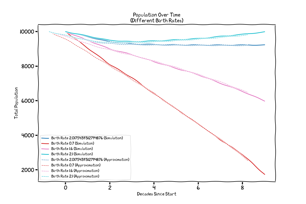
Figure 10. Population over time simulated vs. approximated.

The following shows the quality of the approximation looking at simulated populations over time by age bracket. This approximation is only good for brackets up to $60$ years as afterwards the mortality rates play a significant role which are not included in the approximation based on birth rates.

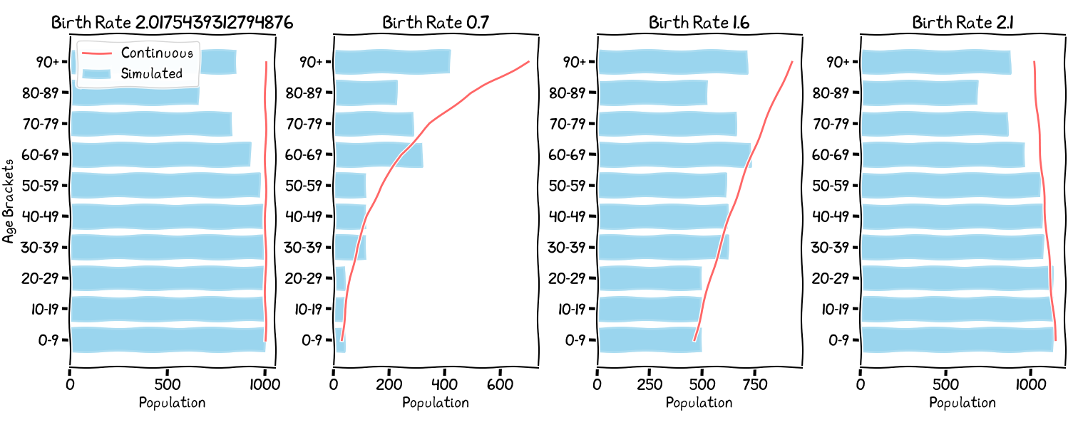
Figure 11. Birthrate vs. population size simulated vs. approximated.

Understanding Age Dependency Ratios in Population Dynamics

In demographic studies, the age dependency ratio is a crucial metric that helps us understand the economic implications of population changes. This ratio provides insight into the balance between the dependent population and those typically in the workforce. Understanding these ratios is vital for policymakers and economists as they plan for future social services, healthcare, and economic policies. A higher dependency ratio indicates a greater economic burden on the working-age population, which can impact economic growth and the sustainability of social support systems and more generally measure how “close” a population is to the demographic tipping point.

In very general terms the age dependency ratio is given by

\[\tau(x) = \frac{1-x}{x},\]

where $x$ is the proportion of the population that is working-age and $1-x$ the proportion of the population that is dependent. A first very important observation is that the gradient is brutal: $\frac{d\tau}{dx} = - \frac{1}{x^2}$, i.e., the dependency ratio is very sensitive and at high dependency ratios a small reduction in working-age population size or a small increase in dependent population size can lead to a large change in the dependency ratio; see figure below for a visual representation.

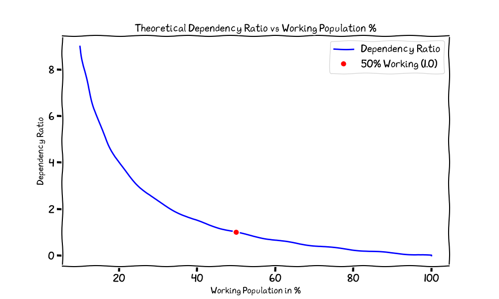
Figure 12. Theoretical dependency ratio.

The dependency ratios are closely related to what we refer to as work attribution (for lack of a better term). It measures how much of the work performed by an individual is attributed to themselves and how much is needed to cover for dependents, i.e., it is defined as

\[w(r) \doteq \frac{1}{1 + r} = x,\]

where $r$ is the dependency ratio and $x$ is the proportion of the population that is working-age, via the formula from above; in fact it is the inverse of the dependency ratio. For example, at a dependency ratio of $0.5$, every working-age person needs to cover for $0.5$ dependents, so that only $0.67$ (two-thirds to be precise) of the work (and the derived benefits) is left for themselves. The following table shows the work attribution for different dependency ratios, and the figure below visualizes the relationship more broadly.

Dependency Ratio (r)	Work Attribution ($1/(1+r)$)
0.1	0.91
0.2	0.83
0.3	0.77
0.4	0.71
0.5	0.67
0.6	0.63
0.7	0.59
0.8	0.56

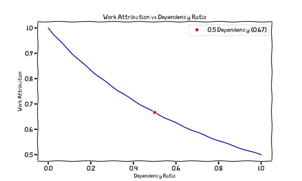
Figure 13. Work attribution vs dependency ratio.

Population Simulation Model

To consider basic mechanics of demographic shifts, we can consider a simple population model. This simulation model is designed to project population changes over time, taking into account birth rates and mortality rates across different age brackets. The model divides the population into ten age brackets, each representing a decade of life, from ages 0-9 to 90+. The model is somewhat simplified and should be interpreted with caution. However, this toy model still captures the basic effects for discussion, albeit with reduced precision. Calibration is against 2023 data from Germany and some assumptions are made for the sake of simplicity. Below we provide some implementation details as they implicitly contain many of the assumptions.

Key Components

Population Update Function:
- The function update_population_with_mortality calculates the new population for each age bracket by applying mortality rates and shifting the population to the next age bracket. New births are calculated based on a specified birth rate and added to the youngest age bracket in the next time step.
Simulation Over Time:
- The simulate_population function runs the population update function over a specified number of years, or time steps, each representing ten years as we shift brackets and a bracket is 10 years. This allows us to observe how the population evolves over time.
Age Dependency Ratio:
- The compute_age_dependency_ratio function calculates the ratio of dependent population (young and elderly) to the working-age population (ages 20-69). This ratio is crucial for understanding the economic implications of demographic changes. We consider age dependency as well as old-age dependency; see below for details. Simulation has been run to steady state to compute the dependency ratios.
Mortality Rates:
- Mortality rates are calculated based on real-world data from German death statistics for 2023.
Simulation Scenarios:
- The model allows for simulations with different birth rates and mortality rates over varying time horizons.

Age Dependency Ratio

The age dependency ratio is calculated by comparing the number of dependents (young and elderly) to the working-age population. In our model, the working-age population is defined as individuals aged 20 to 69, which corresponds to age brackets 2 through 6. These individuals are typically considered to be economically active and are crucial for supporting the dependent population.

Young Dependents: Ages 0-19 (brackets 0-1)
Elderly Dependents: Ages 70 and above (brackets 7-9)
Working Age: Ages 20-69 (brackets 2-6)

The age dependency ratio is calculated as:

\[\text{Age Dependency Ratio} = \frac{\text{Young Dependents} + \text{Elderly Dependents}}{\text{Working Age Population}}\]

This ratio is a key indicator of the economic burden on the working-age population, as it reflects the number of dependents each working individual supports.

Old-Age Dependency Ratio

The old-age dependency ratio focuses specifically on the elderly population, providing a measure of the economic pressure exerted by the aging population on the workforce. This ratio considers only the elderly dependents (ages 70 and above) relative to the working-age population.

\[\text{Old-Age Dependency Ratio} = \frac{\text{Elderly Dependents}}{\text{Working Age Population}}\]

This metric is particularly important in societies with aging populations, as it highlights the potential challenges in providing adequate healthcare, pensions, and social services for the elderly.

A few Comments on Sensitivity

The model’s sensitivity is primarily concentrated in specific age brackets. Birth rates predominantly affect only the first three age brackets (ages 0-29), while mortality rates mainly impact the last three brackets. While these parameters can lead to different dependency ratios, the overall dynamics and trends remain largely similar across reasonable parameter ranges. In particular, the model is relatively insensitive to the actual mortality rates (as long as they are realistic); see figure below for old-age dependency ratio vs birth rates for two mortality rate curves.

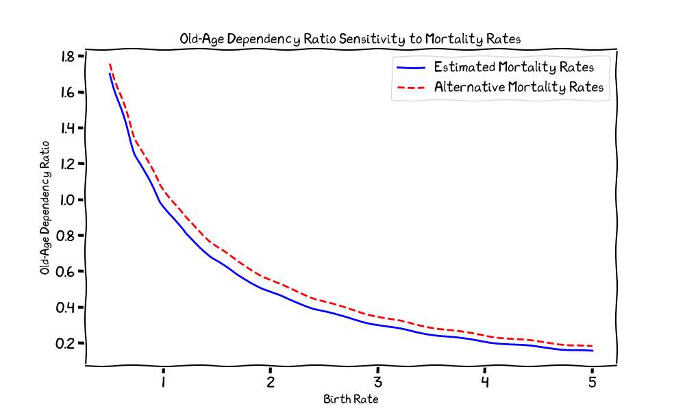
Figure 14. Old-age dependency ratio sensitivity.

It is worth noting that while our model is calibrated approximately for Germany’s demographic data, similar demographic dynamics are observed across most Western countries.

Simulation Results

Here we present some simulation results. The first figure shows the general growth/decline of the population over time as a function of the birth rate. Note that for the first few decades there can be a minor drop although overall the population is stable (for $r$ being the replacement rate) or growing (for $r = 2.1$). This due to the initial population taking on the shape induced by the mortality rates, whereas the birth rate effects only kicks in after three decades.

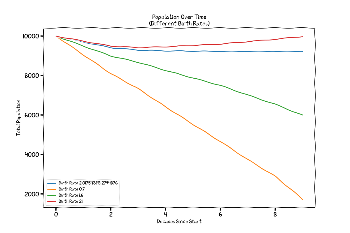
Figure 15. Population over time for varying birth rates.

The following figure depicts the overall structure of the demographic pyramid as function of birth rates for four different scenarios ($r = 0.7$ the “South Korea” scenario, $r = 1.6$ the “Europe” scenario, $r \approx 2.01$ being the replacement rate, and $r = 2.1$ the “slight growth” scenario). We also report the induced age dependency ratios for the respective scenario.

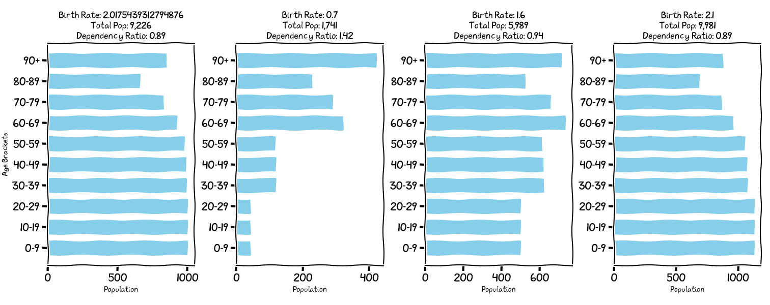
Figure 16. Population pyramid for varying birth rates with age dependency ratios.

Same as above but for the old-age dependency ratio.

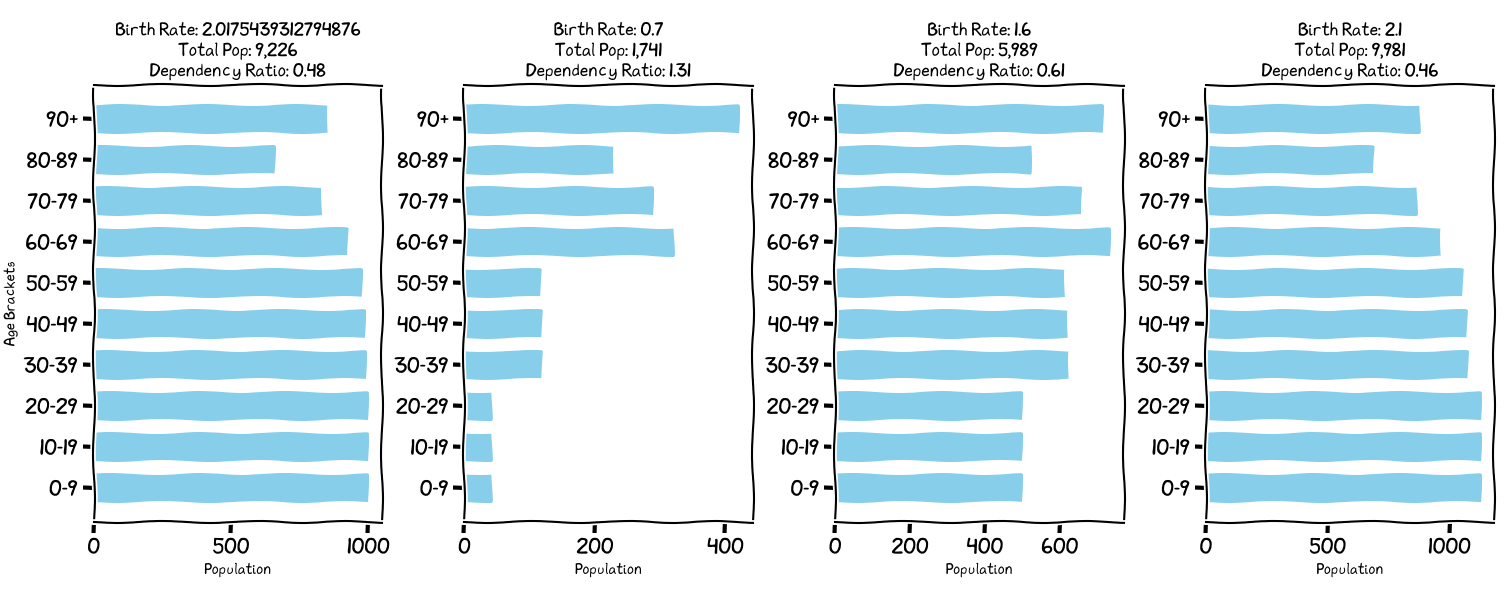
Figure 17. Old-age dependency ratio for varying birth rates with old-age dependency ratios.

The next figure more generally shows age dependency ratios for varying birth rates obtained from the simulation. As mentioned above this done for the mortality rates roughly calibrated to the German data for 2023 but holds more widely. Note that this curve actually has a minimum at around $r = 2.39$ as beyond the point we have increased dependency from young dependents. For reference the value of $1.01$ for Germany with $r = 1.32$ (via the 2023 data) has been added. Note that this is considerably higher than the minimum value of $0.88$ for $r = 2.39$.

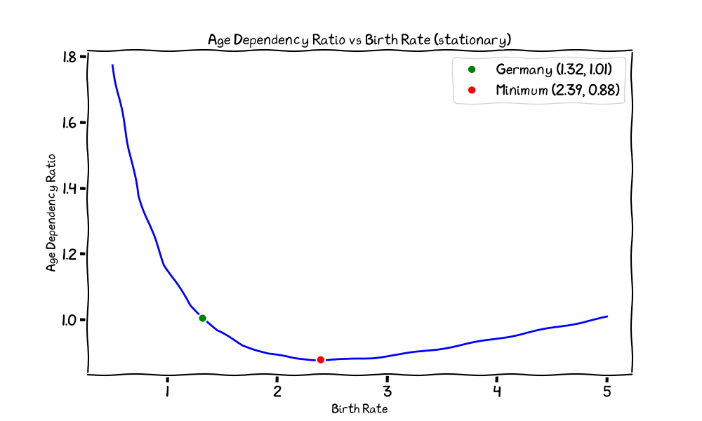
Figure 18. Age dependency ratios for varying birth rates.

The next figure shows the old-age dependency ratios for varying birth rates. Here there is no minimum as higher birth rates lead to lower old-age dependency ratios. This however implies or assumes an ever-growing population size which is not realistic if the rate is too high. As before we added the value of $0.74$ for Germany with $r = 1.32$ for reference, which is considerably higher than the value of $0.48$ for $r$ being the replacement rate.

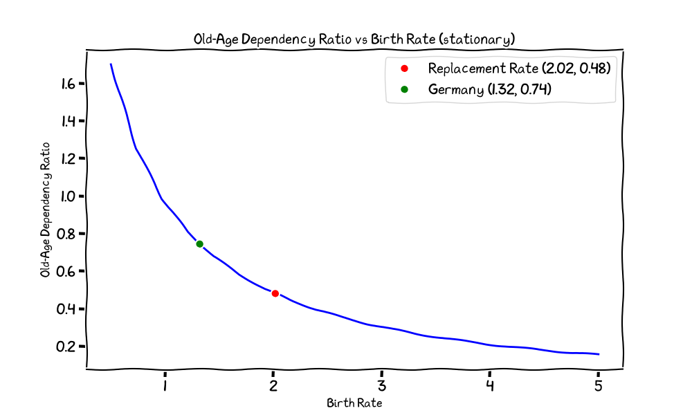
Figure 19. Old-age dependency ratios for varying birth rates.

Disaggregated Total Fertility Rates

The decomposition of the Total Fertility Rate (TFR) into the Total Maternal Rate (TMR) and Children per Mother (CPM)—as formalized by Shaw (2025)—clarifies two distinct components of fertility behavior that are otherwise merged in the traditional single-index TFR. Mathematically,

\[\text{TFR} = \text{TMR} \times \text{CPM},\]

where TMR measures the proportion of women who become mothers (the societal likelihood of motherhood), and CPM measures the average number of children among mothers. This decomposition enables demographers to separate entry into motherhood from family size among mothers, providing a clearer view of whether fertility decline stems from increasing childlessness or smaller families. The framework aligns with period-based data rather than retrospective cohort studies, allowing for timely analysis of current fertility trends.

The usefulness of this decomposition lies in its ability to recover information that is lost when TFR is used alone. Shaw’s analysis across 33 economies found that aggregating TMR and CPM into TFR causes a 48.9 % loss of informational entropy, meaning that TFR retains only about half of the statistical information contained in its components. Furthermore, TMR and CPM were found to be statistically independent—each shaped by distinct social and economic factors—so combining them obscures independent trends. For instance, periods where motherhood rates drop but family sizes remain stable (or rise) are invisible in the aggregate TFR. Empirically, models that include both TMR and CPM gain an average of +0.385 in adjusted R² over TFR-only models, underscoring their superior explanatory power.

However, while decomposition increases interpretability, it also highlights data loss inherent in the TFR as a summary measure. Because many different combinations of TMR and CPM can yield the same TFR value, a single TFR (e.g., 1.5) may correspond to a wide range of underlying demographic realities—different balances of childlessness and family size. This ambiguity limits the TFR’s usefulness for cross-national comparison and policy design. The microdemographic decomposition thus preserves more information, reduces interpretive error, and transforms fertility measurement from a descriptive average into a diagnostic tool for understanding real-time reproductive behavior.

Remark. The claimed 48.9% loss of informational entropy is buggy as they used Pippenger’s bound but this is for continuous derivations. However, they discretize their data into buckets. For discrete random variables the loss is a little smaller (in fact only 1 bit for optimal coding in contrast to 1 nat for the continuous case) as we explain, so that the actual information loss is even higher.

Discrete Aggregation: Clean, Rigorous Proof (Uniform RVs)

Let $X,Y$ be independent and uniform on ${1,\dots,n}$. Let $W\doteq (X,Y)$ so $\lvert\mathcal W\rvert=n^2$ and $H(W)=\log_2(n^2)=2\log_2 n$. Let $Z=f(W)$ be any deterministic aggregation. For each $z$, define the fiber multiplicity

\[m(z)\doteq \bigl|\{\,w\in\mathcal W:\ f(w)=z\,\}\bigr|.\]

Then $\sum_{z} m(z)=n^2$ and $p_Z(z)=m(z)/n^2$.

Theorem (Exact loss = expected log multiplicity).

The information loss

\[L \stackrel{\mathrm{def}}{=} H(W)-H(Z) = H(W\mid Z)\]

satisfies the exact identity

\[L = \mathbb{E}_Z[\log_2 m(Z)] = \frac{1}{n^2}\sum_{z} m(z)\,\log_2 m(z)\]

Proof.
Compute $H(Z)$ from the pushforward probabilities:

\[H(Z) = -\sum_z \frac{m(z)}{n^2}\log_2\left(\frac{m(z)}{n^2}\right) = -\frac{1}{n^2}\sum_z m(z)\log_2 m(z) + \frac{1}{n^2}\sum_z m(z)\cdot \log_2(n^2).\]

Since $\sum_z m(z)=n^2$ and $H(W)=\log_2(n^2)$,

\[H(Z) = \log_2(n^2) - \frac{1}{n^2}\sum_z m(z)\log_2 m(z).\]

Thus

\[L = H(W)-H(Z) = \frac{1}{n^2}\sum_z m(z)\log_2 m(z) = \sum_z \frac{m(z)}{n^2}\log_2 m(z) = \mathbb{E}_Z[\log_2 m(Z)]. \quad \square\]

Corollary (Optimal coding; balanced fibers).

Among all deterministic $f$ with fixed output alphabet size $k=\abs{\mathcal Z}$, the loss $L$ is minimized when fibers are as equal as possible:

\[m(z)\in\{\lfloor n^2/k\rfloor,\ \lceil n^2/k\rceil\}\quad\text{for all }z.\]

If $k\mid n^2$ (perfectly balanced), then

\[m(z)=\frac{n^2}{k}\ \forall z,\qquad H(Z)=\log_2 k,\qquad L_{\min}=\log_2\left(\frac{n^2}{k}\right).\]

Proof.
Since $x\mapsto x\log x$ is convex, $\sum_z m(z)\log m(z)$ is minimized (for fixed $\sum_z m(z)=n^2$) by equal $m(z)$ up to rounding (Jensen/Karamata). Substitute into the theorem. $\square$

Remark (1-bit loss case: balanced 2-to-1).

If every fiber has size $m(z)=2$ (i.e., $k=n^2/2$), then

\[L = \log_2 2 = 1\ \text{bit.}\]

This is tight and attained by any balanced 2-to-1 partition of the $n\times n$ grid.

Remark.

The discrete, uniform world has no universal constant lower bound;
you can make $L$ any $\log_2(n^2/k)$ by choosing $k$.
The oft-quoted $\log_2 e\approx 1.44$ bits bound is a continuous (differential-entropy) phenomenon;
it does not apply to histogram-discretized entropies without additional limiting assumptions.

The following table summarizes recent micro- and macro-level period-based demographic indicators for selected economies.

Country	Total Maternal Rate (TMR)	Total Childlessness Rate (TCR)	Children per Mother (CPM)	Implied Total Maternal Rate (iTMR = 2.1/CPM)	Children per Woman (TFR)	Year
France	72.8%	27.2%	2.28	92.1%	1.66	2023
Germany	68.3%	31.7%	2.11	99.5%	1.45	2022
Italy	59.5%	40.5%	2.02	104.0%	1.20	2023
Netherlands	66.0%	34.0%	2.18	96.3%	1.44	2023
Japan	58.7%	41.3%	2.13	98.6%	1.25	2022
South Korea	47.9%	52.1%	1.75	120.0%	0.84	2020
Spain	57.5%	42.5%	1.95	107.7%	1.12	2023
Turkey	62.0%	38.0%	2.60	80.8%	1.61	2022
United Kingdom	70.5%	29.5%	2.23	94.3%	1.57	2020
United States	63.6%	36.4%	2.61	80.5%	1.66	2021

Table. Recent micro- and macro-level period-based demographic indicators for selected economies. iTMR = 2.1 / CPM is the implied maternal rate required to reach replacement fertility (TFR ≈ 2.1); values above 100% indicate replacement is unattainable without higher CPM.

This in particular shows 3 types of economies:

Those where the CPM is less than replacement: Here even a 100% TMR would not be enough to sustain the population. This includes Italy, South Korea, Spain
Those where the CPM is roughly equal to replacement: A conservative estimate of involuntary childlessness is about 5%-10% (depending on statistics). Assuming 5% everything with iTMR > 95% is infeasible. This includes Germany, Netherlands, Japan, United Kingdom, United States.
Those where the CPM is so high that at very high TMRs it is still possible to sustain the population. This includes France, Turkey, United Kingdom (barely), and United States.

And only Turkey and the United States have family sizes large enough to require iTMRs of only around 80%. Note that even in those cases the rates are high, requiring (on average) 4 out of 5 women to become mothers throughout their lives.