The Basics of Compounding
TL;DR: In this post we look at very simple consequences of compounding and what it means for investing. Just basic maths and actual historic numbers. If you do not know why you are here you are probably not meant to; there is a reason why this post is not linked.
Note. The following does not constitute investment or tax advice.
This post is about the basics of compounding. While most of us do understand exponential growth and geometric series on paper in an abstract fashion, here we will try to take a more tangible look using somewhat realistic assumptions, or at least a set of assumptions that are consistent with historical data in the context of capital growth. There is nothing special happening here, just simple math with actual numbers.
Interlude. What do I mean by consistency? Very hand-wavy, the Anthropic Principle applied to the market: conditions and rates observed by us have to be compatible (1) with us being able to observe them, as well as (2) the average human life expectancy, and (3) the general state of society. For example, general market growth rates of $30\%$ throughout and consistently over decades seem unrealistic as production, value, etc would have to double about every $2.5$ years.
Getting some things out of the way
We will now explain assumptions and scope. Our basic assumption is that we consider compounding return models, i.e., given some annual rate of return $r$ and some investment period $T$, then our initial investment, which we assume (without loss of generality) to be $1$ throughout, grows as:
\[(1+r)^T.\]Continuous vs. discrete compounding
In the above and the following we will use discrete compounding with annual rates, i.e., we compound as $(1+r)^T$; other time intervals follow simply by rescaling rates etc. The mathematically somewhat cleaner model is the continuous compounding model where $r$ is not an annual rate of return but rather the continuous spot rate, so that we compound as $e^{rT}$. However, these two models only differ in the effective rate, as we can simply rewrite
\[(1+r)^T = e^{T \log (1+r)},\]i.e., for the annual rate of return $r$ the corresponding spot rate is simply $\log (1+r)$, where $\log$ is the natural logarithm throughout. As most reported rates are reported as annual rates of return we will stick to the discrete (annual) compounding model if not stated otherwise.
We hasten to stress to not equate the spot rate and the annual rate of return. While $\log (1+r) \approx r$ for small $r$, generally we only have $\log (1+r) \leq r$ and in fact the approximation error can be quite pronounced over longer investment horizons as we see in the following figure:
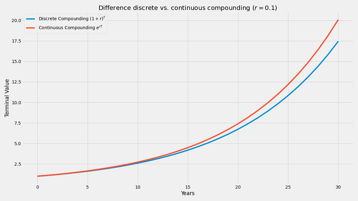
Figure 1. Discrete Compounding with an annual rate of 10% vs. Continuous Compounding with a spot rate of 10%
Inflation
In the following we do not explicitly deal with inflation. However, at the end of the day inflation is affecting the effective rate at which we compound and it can either be applied at the end at time $T$ to the total capital or by reducing the rate. Suppose the annual inflation is denoted by $\gamma$, we have an annual rate of return of $r$ and we are investing for a time period $T$. Starting with one unit of capital at $t=0$, we have, before accounting for inflation, a total capital of $(1+r)^{T}$ at time $T$ and after accounting for inflation, we have:
\[(1+r)^{T} \cdot (1-\gamma)^{T} = ((1+r) (1-\gamma))^T = (1 + r - \gamma - r\gamma)^T,\]i.e., either we discount the final value with $(1-\gamma)^{T}$ or we adjust the rate from $r$ to $r - \gamma - r\gamma$.
NB. Things are slightly nicer in continuous discounting. Here we compound before inflation at $e^{rT}$ and after inflation at $e^{(r-\gamma)T}$.
A “reasonable” value for $\gamma$ is somewhere between $2\% - 3\%$; see the following figure. As a consequence of the stimulus measures to combat the economic impact of the COVID-19 pandemic expect values on the higher end (or even much higher; who knows) in the near to midterm future.
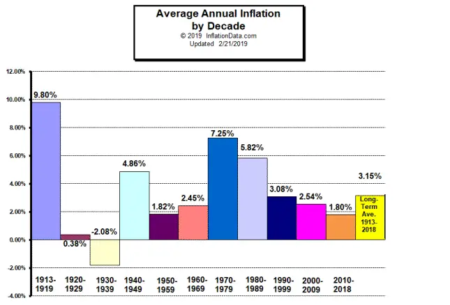
Figure 2. Historic US inflation levels (Source: InflationData).
Scope
The scope of this post is really on the macro level and we are not going to dive into micro level specifics such as wash-sale rules, offsetting capital gains with losses for tax purposes, tax mechanics of specific countries and their capital gain taxation rules (except for some very basic macro impacts), investment mechanics for specific countries, asset or security selection etc. Let me stress this once more:
The following does not constitute tax or investment advice. Please consult with your CPA or financial advisor for your specific situation.
Basic guiding principles for the average retail investor
The following „basic rules“ are all to be taken with a grain of salt and are to be considered as mere rules-of-thumb. Exceptions are very well possible, but you should have a very good reason why you think you know something that others don‘t:
If you cannot spot the sucker in the room, it is you.
So here we go:
- Don‘t try time the market.
- Don‘t try to predict prices.
- The market can stay longer irrational than you can stay liquid.
- Trading turns an information advantage into a dollar advantage: no information advantage means no trading advantage (and that is before fees, spreads, etc).
Beyond that, more generally:
- You need to understand the specifics of taxation. This is not minor.
- You need to have proper accounting of investments, gains, and losses. Preferably double-entry to simplify analyses of cashflows etc.
These two things can easily turn a seemingly unfavorable investment into a favorable one, due to offsetting some of the gains or exemption from taxes. One specific example is the difference in treatment of crypto assets between the US and Germany; the former considers it an asset with the usual capital gain taxation structure, the latter consider it as art with tax exemptions for gains after a certain holding period; as before: no tax advice but simply pointing out differences in different jurisdictions.
Basic rules of compounding
Having all that out of the way let us get started. The following table shows nominal annualized returns for global stocks from 1900 - 2019 for some select countries (Source: Mindfully Investing) as well as the one-time vs. recurrent equivalency factors, which we will explain, derive, and discuss further below.
| Country | Returns | Factor |
|---|---|---|
| USA | 9.4% | 11.64 |
| Germany | 6.5% | 16.38 |
| UK | 8.1% | 13.35 |
| Europe | 7.2% | 14.89 |
| World | 8.0% | 13.50 |
As we can see historically equity return rates have been hovering somewhere between 9.4% (US) on the high end and 6.5% (Germany) on the low end with a worldwide average of 8.0%.
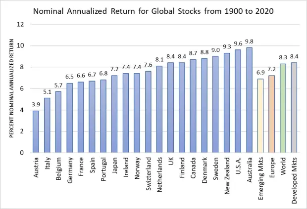
Figure 3. Historic global returns from 1900-2019 (Source: Mindfully Investing).
Keep also in mind that it might be helpful to consider inflation-adjusted returns here. With the comment from before this effectively amounts to subtracted a suitable inflation rate, say 3%. Then Germany’s return drops to 3.5% and the US return to 6.4%; about twice as high. This is not a subtle difference: $e^{rT} = e^{(r/2)\cdot (2T)}$, i.e., halving the rate means that it takes twice as long to reach the same terminal wealth.
One-off investments
We first consider the basic case of a one-off (or one-shot) investment, i.e., say investing USD 10k today.
Time-to-double and Time-to-10x
Two very handy measures for quick estimations of growth are time-to-double and time-to-10x. We simply have that
\[(1+r)^t = 2 \Leftrightarrow t \log 1+r = \log 2 \Leftrightarrow t = \frac{\log 2}{\log 1+r}.\]This gives us the time-to-double $T_2(r)$ for a given rate $r$ as $T_2(r) = \frac{\log 2}{\log 1+r}$ and similarly a time-to-10x $T_{10}(r)$ as $T_{10}(r) = \frac{\log 10}{\log 1+r}$.
Assuming that rates $r$ are reasonably small we can use the approximation $\log 1+r \approx r$ and further $\log 2 \approx 0.6931$ and $\log 10 \approx 2.3026$ so that we get the rough rules-of-thumb, which are good enough for most back-of-the-envelope estimations:
\[\tilde T_2(r) = \frac{69}{r \cdot 100} \qquad \tilde T_{10}(r) = \frac{230}{r \cdot 100},\]where the multiplication with $100$ is simply to indicate that we divide by the “percentage number”, i.e., if $r=10\% = 0.01$, we would divide by $10$. The following table reports exact growth factors as well as those from the approximations:
| $r$ | $T_2$ | $\tilde T_2$ | $T_{10}$ | $\tilde T_{10}$ |
|---|---|---|---|---|
| 0.01 | 69.66 | 69.00 | 231.41 | 230.00 |
| 0.02 | 35.00 | 34.50 | 116.28 | 115.00 |
| 0.05 | 14.21 | 13.80 | 47.19 | 46.00 |
| 0.07 | 10.24 | 9.86 | 34.03 | 32.86 |
| 0.10 | 7.27 | 6.90 | 24.16 | 23.00 |
| 0.12 | 6.12 | 5.75 | 20.32 | 19.17 |
Impact of Capital Gain Tax
The basic rule of thumb is, whenever you sell an asset you will (likely) have to pay capital gain taxes on the gains (only) and not on the principal assuming that the principal was invested post-tax or taxation is deferred etc e.g., in a 401k with pre-tax contributions. Invested (non-deferred) pre-tax contributions or principal are likely going to be taxed also. The specifics are beyond the scope but you should check beforehand to understand the exact taxation rules.
For the sake of exposition here, we assume that the principal is not subject to capital gain taxes. In our language the total value at time $T$ is $(1+r)^T$ and the gain is $(1+r)^T - 1$. Why is this important? Every time you sell an asset in order to rebalance, the capital gain taxes effectively reduce your gains and hence the effective rate of return. When considering large investment horizons $T$, capital gain tax is not as bad as inflation as it is one-off whereas inflation compounds; the situation is different if you regularly rebalance as this turns the one-off capital gain tax into a compounding one as we will see in the next section.
A good perspective on capital gain taxes is how many years of investing/compounding are lost due to capital gain taxes. Suppose a capital gain tax of $\mu$, then we solve the following identity for $\Delta$:
\[(1-\mu) \cdot ((1+r)^{T} - 1) + 1 = (1-\mu) \cdot (1+r)^{T} + \mu = (1+r)^{T-\Delta},\]where $\Delta$ is then the number of years we lost. Ignoring the additive $\mu$ term as it will be relatively small in the long run and estimating more conservatively that way, the above leads to:
\[(1-\mu) = (1+r)^{-\Delta} \Leftrightarrow - \frac{\ln (1-\mu)}{\ln (1+r)} = \Delta,\]which we depict in the next figure for various capital gain tax rates and return rates.
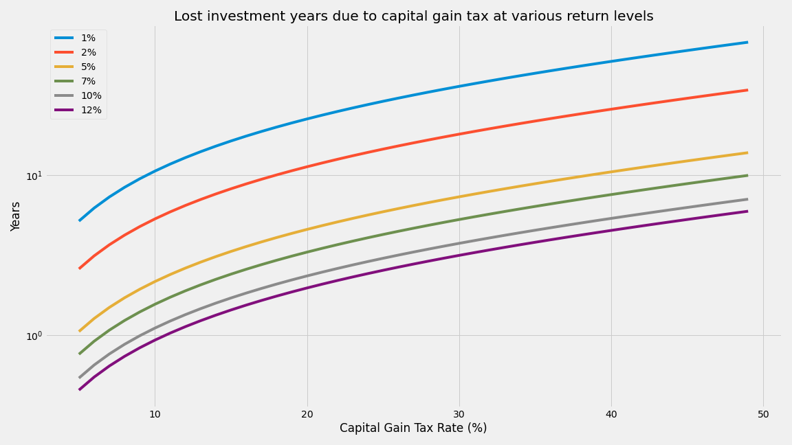
Figure 4. Lost investment years due to capital gain tax. The lines corresponds to different rates of return and the x-axis represents the capital gain tax rate. The y-axis is the number of lost investment years (in log-scale).
At historic return rates from above and the prevalent capital gain tax rates, in the US this comes down to around 2.483 years whereas in Germany this comes down to 4.86 years, so that in most scenarios the loss of investing years due to capital gain taxes is somewhere between 2.5 - 5 years. Put more bluntly, as a rule-of-thumb, over longer investment horizons, about 2.5 - 5 years are lost due to capital gain taxes.
Impact of Capital Gain Tax when Rebalancing
When it comes to rebalancing the situation gets significantly worse if we rebalance relatively often as in this case the one-time capital gain tax that we would pay at the end when realizing the investment, effectively turns into something like a compounding tax. This significantly impacts our effective rates of return as we will see now. As such it is important to consider the trade-off of extra return due to rebalancing vs. reduced return due to triggered capital gain taxes.
The general model that we are operating under is that at time of selling/rebalancing we trigger a capital gain tax event, effective reducing the gain. This is a reasonable assumption for most retail/private investors; as mentioned above, for specific retirement constructs capital gain taxation might be reduced or deferred and checking the rules is imperative. For the sake of simple exposition we assume that the whole position is liquidated and reinvested. Clearly the same arguments apply to partial rebalancing with the corresponding rescaling and finer accounting.
If we invest for a time period of $T$ at an annual rate of $r$ and captial gain tax of $\mu$, we have a post-tax capital at time $T$ of:
\[1 + ((1+r)^{T}-1) (1-\mu) = (1+r)^{T} (1-\mu) + \mu,\]where we have the additional $1$ for our non-taxed principal and the subtraction of that same one from the total pre-tax capital of $(1+r)^T$, whose gains are subject to capital gain taxation.
Now let us assume that we rebalance $K$ times, say evenly distributed across the time horizon $T$. We then have a terminal post-tax capital as follows, which, for $K$ tending to $\infty$, converges to:
\[((1+r)^{T/K} (1-\mu) + \mu)^K \stackrel{K \rightarrow \infty}{\longrightarrow} (1+r)^{(1-\mu)T},\]and lends itself to two perspectives: (a) either a reduced rate factor from $(1+r)$ to $(1+r)^{(1-\mu)}$ or (b) reduced investment horizon from $T$ to $(1-\mu)T$. Put differently, frequent rebalancing can turn the one-time multiplicative loss of capital gain tax into a much worse reduction in effective rate or investment horizon, so that any rebalancing strategy has to compensate for that loss in the limit to make sense.
So how bad is it in practice? Now let us assume that we rebalance $K$ times, say evenly distributed across the time horizon $T$. We then have a terminal post-tax (annual) rate of return of:
\[((1+r)^{T/K} (1-\mu) + \mu)^{K/T}.\]The following graph depicts the reduction in effective rate as a function of number of rebalancing operations. As we can see, we are quite close to the “limit” from above already after about 10 times rebalancing over a horizon of 30 years; the rebalancing operations are spread out evenly in time.
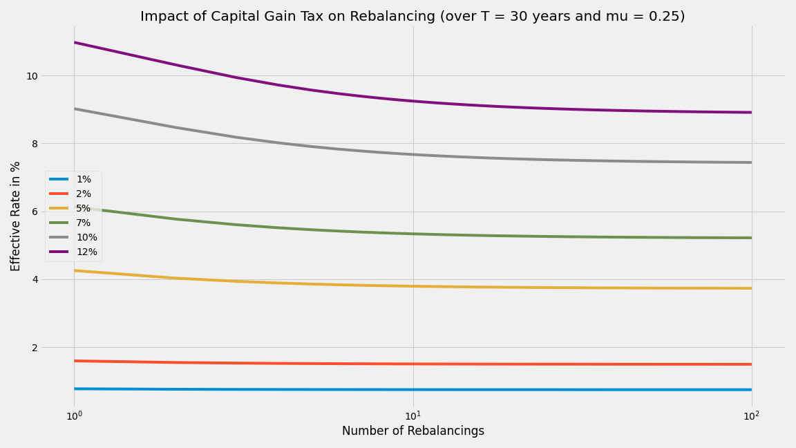
Figure 5. Impact of number of rebalancing operations (on x-axis) on return rates (on y-axes) for various return rates with $\mu = 0.25$.
The special case $K = T$. This happens in the context of (annual) dividend reinvesting. We have:
\[((1+r)^{T/K} (1-\mu) + \mu)^K = ((1+r) (1-\mu) + \mu)^T = (1 + r(1-\mu))^T.\]Calculation of limit. The above limit follows from considering the continuous compounding variant and computing the limit:
\[(e^{rT/K} (1-\mu) + \mu)^K \stackrel{K \rightarrow \infty}{\longrightarrow} e^{(1-\mu)rT},\]which is then transformed back to the discrete compounding case.
As such as, as a rule-of-thumb, you need to improve your return from $r$ to at least $r/(1-\mu)$ via rebalancing to at least break even and that is only for the case of relatively infrequent rebalancing once a year. No small feat given prevalent return rates and capital gain tax rates.
Continuous investing
Realistically, in many real-world scenarios apart from investing a relatively large sum one time, the other realistic model is to make regular contributions to your investments at regular intervals, e.g., say USD 1000 each month.
Dollar-cost averaging
While dollar-cost averaging (DCA) might be a controversially discussed strategy with lots of misunderstandings and concept creep, at the end of the day this is what many retail investors end up doing naturally by their usual real-world operating constraints: at the end of each month they invest a set amount of money. So let us understand the rough return to be achieved by dollar-cost averaging (for the less stars-and-stripes minded: unit-cost averaging). Let $p_T$ denote the price of an asset at time $T$ and $p_h$ be the harmonic mean of prices at each buying event, then we have in our language here $(1+r)^T = \frac{p_T}{p_h}$.
Reinvesting of dividends
Several stocks pay dividends with some dividend rate $r$; the actual rate might depend on various conditions. A natural thing is to reinvest the dividend back into the same stock to grow the holding of the stock. What is important to keep in mind is that there are usually tax implications of dividends, e.g., often they are taxed similar to capital gains, effectively reducing the growth factor from $(1+r)$ to $(1+r (1-\mu))$ (in the discrete compounding model), so that after time $T$ we have a terminal wealth of $(1+r (1-\mu))^T$, i.e., the dividend rate is effectively reduced by the tax rate. On the other hand, observe that the reinvesting here effectively might turn a stock that has been traditionally flat but paid a dividend into an investment with geometric growth (provided (1) the dividend rate stays the same, (2) the value of the asset is not declining etc, and (3) we are not hitting the limit of available stock).
Save-and-Compound
We will now consider the more common setup where a specific amount of capital is regularly invested, e.g., each month or each year: at each time interval a fixed amount $K$ is invested and compounds at a fixed rate $r$. This will lead us to the save-and-compound model. This model is of particular interest as it nicely captures what I call the arithmetic-geometric-crossover: at the beginning it is the arithmetic growth that dominates the growth, i.e., the regular investments that we make. Further down the road however, it is the geometric growth from compounding that takes over.
What do I mean by this? Before looking at the math, let us consider the simple example of investing one unit of capital each year without any compouning. Then after year 1, we have $1$ unit (or infinite growth from $0$ to $1$), after year 2, we have $2$ units (or $1/1 = 100\%$ growth), after year 3, we have $3$ units (or $1/2 = 50\%$ growth), and so on: after year $t$ we have a growth of $1/t$. So in the early years the growth from “saving” (additive growth) is very large but it drops at a rate of $1/t$ converging to $0$ in the long run. On the other hand, geometric growth where our wealth grows as $(1+r)^t$ is very slow in the beginning but very pronounced in the long run. What if we could combine the two effects? This is exactly what the save-and-compound approach does.
NB. For the optimizers in the know, this is nothing else but the same crossover that happens in geometric scaling, bit scaling, or more generally restart strategies. For example, in the smooth convex case, you can obtain a linear rate of convergence of the form $e^{-rt}$ from a sublinear one of the form $1/t$ by means of restarting the $1/t$ convergence sequence provided one knows the strong convexity constant; this is exactly the same mechanic here, if you wrote down the right problem/algorithm; see [P] for an overview of restarting. Put differently, the save-and-compound strategy is a simple restart strategy. Also here it is important to understand that in the early iterations, the linear rate that is valid in the long run is typically dominated by the sublinear rate; simply because $(1-1/t) \leq (1-\mu/L)$ for $t$ small, hence we contract faster in the beginning.
In the following, for simplicity, let us assume that our investment interval is annual and we report end-of-the-year wealth. In the save-and-compound setup our wealth grows then as a geometric series of the form
\[\sum_{t=1}^{T} a^t = \sum_{t=0}^{T-1} a^{t+1} = a \sum_{t=0}^{T-1} a^t = a \frac{1-a^{T}}{1-a} = (1+r) \frac{(1+r)^{T}-1}{r},\]with $a = (1+r)$ and $r$ is the annual return on the already invested capital.
So what does this mean in actual numbers? See the following figure and table below:
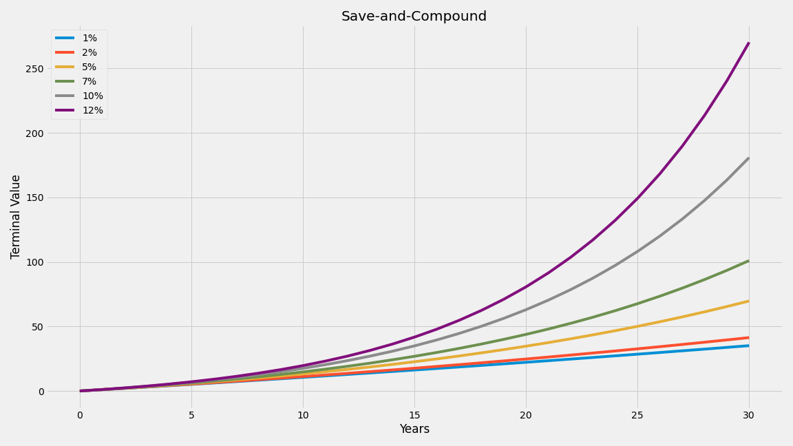
Figure 6. Save-and-compound growth rates and terminal wealth factors assuming annual investment of one unit of capital.
| Years/Rates | $1\%$ | $2\%$ | $5\%$ | $7\%$ | $10\%$ | $12\%$ |
|---|---|---|---|---|---|---|
| 5 | 5.15 | 5.31 | 5.80 | 6.15 | 6.72 | 7.12 |
| 10 | 10.57 | 11.17 | 13.21 | 14.78 | 17.53 | 19.65 |
| 15 | 16.26 | 17.64 | 22.66 | 26.89 | 34.95 | 41.75 |
| 20 | 22.24 | 24.78 | 34.72 | 43.87 | 63.00 | 80.70 |
| 25 | 28.53 | 32.67 | 50.11 | 67.68 | 108.18 | 149.33 |
| 30 | 35.13 | 41.38 | 69.76 | 101.07 | 180.94 | 270.29 |
The effect is quite pronounced. For example at, say $7\%$ annual return over $20$ years of saving-and-compounding we will have grown our wealth by a factor of about $44$. This would be the equivalent of vanilla saving of one unit of capital for $44$ years, i.e., we “doubled” the effective time we have been saving by exploiting the compounding effect.
Save-and-Compound vs. One-shot investment
There is also a certain equivalence that allows to compute the equivalent value of a save-and-compound strategy run ad infinitum in terms of a one-shot investment at time $t = 0$ (i.e., investing a fixed sum and then just let it compound) assuming identical rates etc.
For this we revisit our formula from above, substitute $a = 1+r$, and rewrite to obtain:
\[\sum_{t=1}^{T} (1+r)^t = (1+r) \frac{(1+r)^{T}-1}{r} = (1+r)^{T} \frac{(1+r) - \frac{1}{(1+r)^{T}}}{r} \approx (1+r)^{T} \frac{(1+r)}{r},\]where the last approximation hold in the long run as $\frac{1}{(1+r)^{T}} \stackrel{T \rightarrow \infty}{\longrightarrow} 0$. Therefore a recurrent save-and-compound investment of $1$ unit is (in the long run) equivalent to a one-shot investment of $\frac{(1+r)}{r}$ units.
Before we look at a few specific examples to better grasp the numbers, let us first consider how good that approximation is. In fact, for short time horizons and in particular small $r$ it is not that great. This is due to the fact that the one-shot investment compounds on its full principal from the start, whereas the save-and-compound strategy needs to build up momentum first.
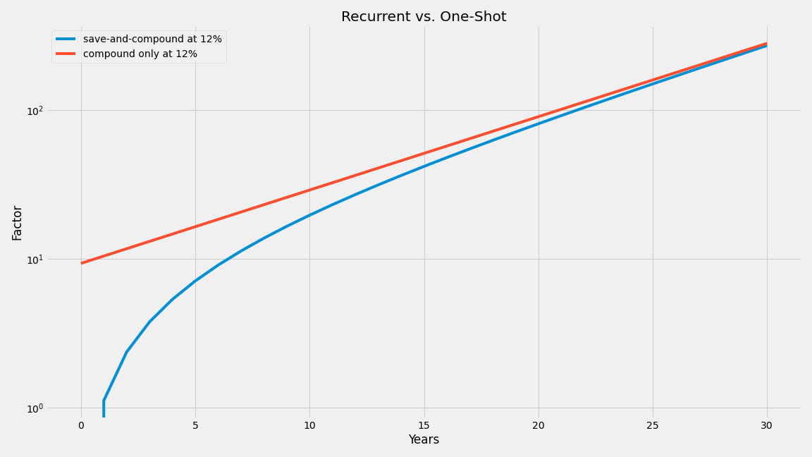
Figure 7. Return factor of save-and-compound of $1$ unit vs. one-shot investing of $\frac{(1+r)}{r}$ units over time with $r = 12\%$.
To give a slightly more complete picture in terms of the error of the approximation, the following figure depicts the ratio of save-and-compound vs. one-shot (with the rescaling of $\frac{(1+r)}{r}$) for various rates $r$ over time.
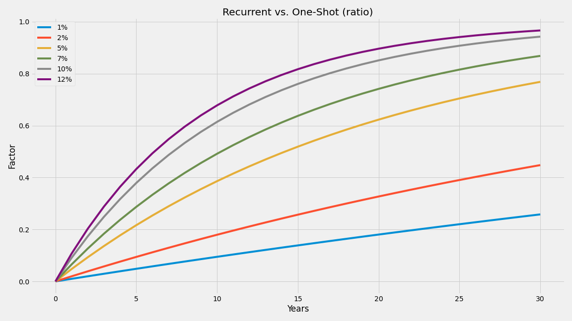
Figure 8. Ratio of the save-and-compound vs. one-shot (with the rescaling of $\frac{(1+r)}{r}$). In the long run the ratio converges to $1$ in all cases, however in the short run the difference can be pronounced.
So as a rule-of-thumb, after about 20 years of investing for prevalent long-term rates the save-and-compound strategy provides a return factor of at least $80\%$ of that of the rescaled one-shot strategy (with the appropriate rescaling factor $\frac{(1+r)}{r}$).
So why did we compute the rescaling factors in first place? To be able to compare investments against the one-shot (or equivalently buy-and-hold) strategy. The scaling factor $\frac{(1+r)}{r}$ for the respective countries is given in the last column in the return table provided at the beginning. For example in the US the factor is roughly 11.64. So if you inherit, say \$1m and invest it this is equivalent (and in fact better in the early years) to saving-and-compounding about \$86k every year for the rest of your life. This provides some perspective.
Geometric Series and Expansion Factors
We encounter geometric series of the form \(\sum_{t=1}^{T} (1+r)^t\) in many contexts. It holds:
\[\sum_{t=1}^{T} (1+r)^t = (1+r) \frac{(1+r)^{T}-1}{r} = \frac{(1+r)^{T+1}-1}{r} - 1 = \frac{(1+r)^{T+1}}{r} - \frac{1+r}{r}.\]If \(r=0\) we have \(\sum_{t=1}^{T} 1 = T\). The additional gain from the interest expressed as factors over \(T\) we call the expansion factors and is given by the ratio of the sum of the series to the number of terms, i.e.,
\[\frac{\sum_{t=1}^{T} (1+r)^t}{T} = \frac{(1+r) \frac{(1+r)^{T}-1}{r}}{T} = \frac{(1+r)^{T+1}-1}{rT} - \frac{1}{T}.\]For $r$ small we can use the approximation $\log (1+r) \approx r$ to obtain the following approximation:
\[\frac{(1+r)^{T+1}-1}{rT} - \frac{1}{T} \approx \frac{e^{r(T+1)} - 1}{rT} - \frac{1}{T},\]as also used above but note that for larger \(r\) this might be imprecise.
Below we report the (exact) expansion factors for various rates and time horizons.
| Years | $1\%$ | $2\%$ | $5\%$ | $7\%$ | $10\%$ | $12\%$ |
|---|---|---|---|---|---|---|
| 5 | 1.03 | 1.06 | 1.16 | 1.23 | 1.34 | 1.42 |
| 10 | 1.06 | 1.12 | 1.32 | 1.48 | 1.75 | 1.97 |
| 15 | 1.08 | 1.18 | 1.51 | 1.79 | 2.33 | 2.78 |
| 20 | 1.11 | 1.24 | 1.74 | 2.19 | 3.15 | 4.03 |
| 25 | 1.14 | 1.31 | 2.00 | 2.71 | 4.33 | 5.97 |
| 30 | 1.17 | 1.38 | 2.33 | 3.37 | 6.03 | 9.01 |
Mortgages
Note. After having completed a first draft of this section I found a similar blog post on Nick Arnoti’s blog. I took the liberty to incorporate some of this content into this section, in particular the example as well as historical context and the intuition of the Taylor-based approximation; just in case his post is not available in the future. See also his post for a more in-depth analysis of the error from the Taylor-based approximation.
In the following we consider the standard mortgage setup. In a standard mortgage setup, we have the following components: the principal, denoted as \(P\), which is the initial amount borrowed; the periodic interest rate, denoted as \(r_i\); the number of payments, denoted as \(n\); and the fixed payment made each period, denoted as \(M\). With this we can reformulate the balance recurrence as
\[\tag{balanceRecurrence}B_{k} = (1 + r_i)B_{k-1} - M,\]where \(B_{0} \doteq B \doteq P\) and by construction we have \(B_{n} = 0\) as it fully amortizes. The corresponding closed form is given by
\[\tag{balanceClosedForm} \begin{align*} B_{k} &= P(1 + r_i)^{k} - M \sum_{m=0}^{k-1} (1 + r_i)^{m} \\ &= P(1 + r_i)^{k} - M \frac{(1 + r_i)^{k} - 1}{r_i}. \end{align*}\]The interest paid in period \(k\) is given by
\[\tag{interestPaid}I_{k} = r_iB_{k-1},\]and the total interest paid is given by
\[\tag{totalInterest}I = \sum_{k=1}^{n} I_{k} = \sum_{k=1}^{n} r_iB_{k-1}.\]From (balanceClosedForm) we can also derive \(M\) simply by setting \(B_{n} = 0\) and solving for \(M\):
\[\tag{mortgagePayment}M = P \frac{r_i (1 + r_i)^{n}}{(1 + r_i)^{n} - 1} = \frac{P}{n} \underbrace{\left(\frac{n r_i}{1 - (1 + r_i)^{-n}}\right)}_{\doteq E(r_i,n)}.\]In the above we have defined the expansion factor
\[\tag{expansionFactor} E(r_i,n) \doteq \frac{n r_i}{1 - (1 + r_i)^{-n}} \geq 1,\]which measures how much more we pay back in total compared to the initial principal, as \(Mn = P \cdot E(r_i,n)\).
The following table provides the expansion factors for various rates and time horizons with annual payments and compounding.
| Years | $1\%$ | $3\%$ | $5\%$ | $7\%$ | $10\%$ | $12\%$ |
|---|---|---|---|---|---|---|
| 1 | 1.01 | 1.03 | 1.05 | 1.07 | 1.10 | 1.12 |
| 5 | 1.03 | 1.09 | 1.15 | 1.22 | 1.32 | 1.39 |
| 10 | 1.06 | 1.17 | 1.30 | 1.42 | 1.63 | 1.77 |
| 15 | 1.08 | 1.26 | 1.45 | 1.65 | 1.97 | 2.20 |
| 30 | 1.16 | 1.53 | 1.95 | 2.42 | 3.18 | 3.72 |
The same but with monthly payments and compounding:
| Years | $1\%$ | $3\%$ | $5\%$ | $7\%$ | $10\%$ | $12\%$ |
|---|---|---|---|---|---|---|
| 1 | 1.01 | 1.02 | 1.03 | 1.04 | 1.05 | 1.07 |
| 5 | 1.03 | 1.08 | 1.13 | 1.19 | 1.27 | 1.33 |
| 10 | 1.05 | 1.16 | 1.27 | 1.39 | 1.59 | 1.72 |
| 15 | 1.08 | 1.24 | 1.42 | 1.62 | 1.93 | 2.16 |
| 30 | 1.16 | 1.52 | 1.93 | 2.40 | 3.16 | 3.70 |
Note that this makes quite a difference, whether we do annual or monthly payments (and hence compounding).
Note. Before we continue a few remarks are in order:
- In the table above, and more generally here, the number of periods and the interest rate are given in annual terms. Switching to monthly terms is straightforward as we can simply divide the annual rate by 12 and multiply the number of periods by 12; similarly for other compounding periods.
- The table of expansion factors is not symmetric under rescaling in \(r_i\) and \(n\), i.e., \(E(r_i,n) \neq E(2 r_i, n/2)\). For example, with annual compounding, \(E(5\%, 10) = 1.63\) but \(E(10\%, 5) = 1.61\). However, they are usually rather close as we will see below when we consider approximations. In particular, if we switch to monthly rates etc, then the table is (almost) symmetric as we will see below.
Approximations of the Expansion Factor
While an approximation, it is useful to have a simpler formula for intuitive understanding. Using the approximation \(1+r \approx e^r\) for small \(r\) we can use \(1 - (1+r)^{-N} \approx 1 - e^{-rN}\) and define the approximate expansion factor
\[\tag{approxExpansionFactor} \tilde E(r_i,n) \doteq \frac{n r_i}{1-e^{-r_i n}},\]in contrast to the exact expansion factor \(E(r_i,n)\) defined above, the approximate expansion factor \(\tilde E(r_i,n)\) is symmetric in \(r_i\) and \(n\) and in particular under rescaling in \(r_i\) and \(n\), i.e., \(\tilde E(r_i,n) = \tilde E(2 r_i, n/2)\).
| Years | $1\%$ | $3\%$ | $5\%$ | $7\%$ | $10\%$ | $12\%$ |
|---|---|---|---|---|---|---|
| 1 | 1.01 | 1.02 | 1.03 | 1.04 | 1.05 | 1.06 |
| 5 | 1.03 | 1.08 | 1.13 | 1.19 | 1.27 | 1.33 |
| 10 | 1.05 | 1.16 | 1.27 | 1.39 | 1.58 | 1.72 |
| 15 | 1.08 | 1.24 | 1.42 | 1.62 | 1.93 | 2.16 |
| 30 | 1.16 | 1.52 | 1.93 | 2.39 | 3.16 | 3.70 |
At first sight this table does not look that good compared to the exact expansion factor, and considering the error of approximation, i.e., \(\log(E(r_i,n)) - \log(\tilde E(r_i,n)):\)
| Years | $1\%$ | $3\%$ | $5\%$ | $7\%$ | $10\%$ | $12\%$ |
|---|---|---|---|---|---|---|
| 1 | 0.00 | 0.01 | 0.02 | 0.03 | 0.05 | 0.05 |
| 5 | 0.00 | 0.01 | 0.02 | 0.03 | 0.04 | 0.04 |
| 10 | 0.00 | 0.01 | 0.02 | 0.02 | 0.03 | 0.03 |
| 15 | 0.00 | 0.01 | 0.02 | 0.02 | 0.02 | 0.02 |
| 30 | 0.00 | 0.01 | 0.01 | 0.01 | 0.01 | 0.01 |
So the error while small is rather pronounced sometimes, basically whenever the rate is large as expected from the approximation. However, if we switch to monthly rates, i.e., \(r_i \to r_i/12\) and \(n \to 12n\) things considerably improve and in fact this is compatible with how mortgages work, as typically months are considered. For the approximation nothing changes as it is invariant under rescaling, but for the exact expansion factor we obtain a different table:
| Years | $1\%$ | $3\%$ | $5\%$ | $7\%$ | $10\%$ | $12\%$ |
|---|---|---|---|---|---|---|
| 1 | 1.01 | 1.02 | 1.03 | 1.04 | 1.05 | 1.07 |
| 5 | 1.03 | 1.08 | 1.13 | 1.19 | 1.27 | 1.33 |
| 10 | 1.05 | 1.16 | 1.27 | 1.39 | 1.59 | 1.72 |
| 15 | 1.08 | 1.24 | 1.42 | 1.62 | 1.93 | 2.16 |
| 30 | 1.16 | 1.52 | 1.93 | 2.40 | 3.16 | 3.70 |
and associated errors:
| Years | $1\%$ | $3\%$ | $5\%$ | $7\%$ | $10\%$ | $12\%$ |
|---|---|---|---|---|---|---|
| 1 | 0.00 | 0.00 | 0.00 | 0.00 | 0.00 | 0.00 |
| 5 | 0.00 | 0.00 | 0.00 | 0.00 | 0.00 | 0.00 |
| 10 | 0.00 | 0.00 | 0.00 | 0.00 | 0.00 | 0.00 |
| 15 | 0.00 | 0.00 | 0.00 | 0.00 | 0.00 | 0.00 |
| 30 | 0.00 | 0.00 | 0.00 | 0.00 | 0.00 | 0.00 |
which is much better and in fact we can consider them basically being the same.
Note. As the approximate expansion factor is symmetric under rescaling in \(r_i\) and \(n\), we basically obtain via \(\tilde E(r_i,n) = \tilde E(2 r_i, n/2)\), e.g., that a $10$-year mortgage at $5\%$ is equivalent to a $5$-year mortgage at $10\%$ (and vice versa).
From the formula for the approximate expansion factor we can further exploit the symmetry setting \(r_i n = x\) to obtain \(\tilde E(x) = \frac{x}{1-e^{-x}}\). With this we can solve for \(E(x) = 2\) to obtain that for \(x \approx 1.59\) we have \(E(x) \approx 2\). Moreover, this gives rise to another natural approximation via the Taylor series expansion \(\tilde E(x) \approx 1 + \frac{x}{2} + \frac{x^2}{12}\) around \(x = 0\) and we define the Taylor approximation
\[\tag{taylorExpansionFactor} \hat E(r_i, n) \doteq 1 + \frac{r_i n}{2} + \frac{(r_i n)^2}{12},\]Note. The Taylor approximation used above is actually a very good approximation as the full expansion is
\[\tag{fullTaylorExpansion} \tilde E(x) \approx 1 + \frac{x}{2} + \frac{x^2}{12} - \frac{x^4}{720} + O(x^6),\]i.e., the term of order \(3\) is zero.
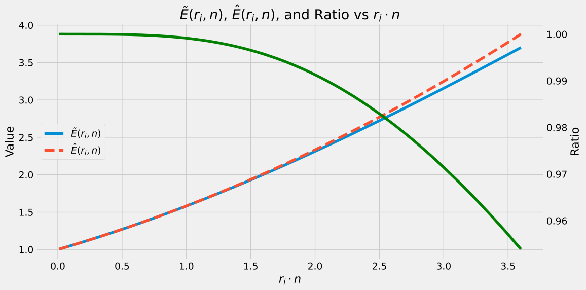
Figure 8. Quality of the approximation of the expansion factor comparing (approxExpansionFactor) (red) and (taylorExpansionFactor) (blue). Ratio of (approxExpansionFactor) to (taylorExpansionFactor) in (green)
Our approximation \(\hat{E}\) consistently overestimates \(\tilde{E}\). When the product \(r_i n\) is small, indicating either low interest rates or short durations, the approximation proves to be highly accurate. Specifically, our approximation remains within 2% accuracy as long as \(r_i n \le 2.6\). For scenarios where \(r_i n\) is larger, an alternative approximation can be employed: \(\tilde{E}(r_i,n) \approx \frac{r_i n}{1-e^{-r_i n}} \approx r_i n\), which tends to underestimate \(\tilde{E}\). By adopting the following estimate:
\[\hat{E}(r_i,n) = \left \{ \begin{array}{l l} 1 + \frac{r_i n}{2} + \frac{(r_i n)^2}{12} & r_i n < 3.3 \\ r_i n & r_i n \ge 3.3 \end{array}\right.\]we can ensure that the approximation remains within 3.7% of \(\tilde{E}\), regardless of the value of \(r_i n\). The accuracy improves significantly when \(r_i n\) is not near the threshold of \(3.3\), which is the case for most situations where \(r_i n < 3.3\).
Summary of the Expansion Factor and Its Approximations
If the discussion above was too long, here is a summary of the key points: The expansion factor \(E(r_i, n)\) is a key quantity in understanding the additional cost of a mortgage. We have derived two approximations to simplify its calculation:
Exact Expansion Factor. (exactExpansionFactor)
\[E(r_i,n) \doteq \frac{n r_i}{1 - (1 + r_i)^{-n}}.\]Approximate Expansion Factor. (approxExpansionFactor)
\[\tilde{E}(r_i, n) \doteq \frac{r_i n}{1 - e^{-r_i n}},\]which is symmetric under rescaling in \(r_i\) and \(n\), i.e., \(\tilde{E}(r_i,n) = \tilde{E}(2 r_i, n/2)\).
Taylor Approximation. (taylorExpansionFactor)
\[\hat{E}(r_i, n) \doteq \left \{ \begin{array}{l l} 1 + \frac{r_i n}{2} + \frac{(r_i n)^2}{12} & \text{if } r_i n < 3.3 \\ r_i n & \text{if } r_i n \ge 3.3 \end{array} \right. .\]In particular, we mostly use \(\hat{E}(r_i, n) \approx 1 + \frac{r_i n}{2} + \frac{(r_i n)^2}{12},\) as for reasonable rates and durations, assuming we use monthly compounding, this is a good approximation.
Example [from Nick Arnoti’s blog]. Let \(P\) be the principal amount you are borrowing, \(r_i\) be your annual interest rate, and \(n\) the number of years that the loan will last.
The first step is to calculate your monthly payment without interest. Take the principal \(P\) and divide it by the total number of payments \(N = 12n\). For example, if you’re borrowing \(\$360,000\) over 30 years (360 months), the monthly payment at a 0% interest rate would be \(\$1,000\). However, the actual monthly payment will be higher due to interest whose effect is captured by the expansion factor \(\hat{E}\), which represents the amount you pay back for every \(\$1\)borrowed: For example, suppose your \(n = 30\) year mortgage has an \(r_i = 5\%\) interest rate. Then \(r_i n = 0.05 \times 30 = 1.5\), and \(\hat{E}(r_i,n) = 1 + \frac{1.5}{2} + \frac{(1.5)^2}{12} = 1.9375\). This indicates that for each dollar borrowed, you will eventually pay back approximately \(\$1.94\).
From this, we can calculate your monthly payment by multiplying \(\hat{E}\) by your interest-free payment. In other words,
\[\hat{M} = \frac{P\hat{E}(r_i,n)}{N} = \frac{P}{12n}\left(1+\frac{r_i n}{2} + \frac{(r_i n)^2}{12}\right).\]For our example with a 30-year loan at 5% interest and a principal of \(\$360,000\), this formula estimates the monthly payment to be approximately \(\$1,937.50\); the calculation via \(\tilde E(r_i/12,12n)\) gives an answer of \(\$1,932.56\), so pretty close as expected, note however that if we would do annual payments that amount would be \(\$1,951.54\), so considerably more. If mortgage rates rise to 7.5%, then \(r_i n = 2.25\), so \(\hat{E}(r_i,n) = 2.547\) and so the monthly payment would be \(\$2,547\); again the exact answer would be \(\$2,517\) so pretty close as expected.
We can also use \(\hat{E}\) for other purposes. For example, \(\hat{E}\) represents \(\$1\) of principal, and the remainder is interest. Thus, your total interest payment is simply
\[\hat{I} = P(\hat{E}-1) = P\left(\frac{r_i n}{2} + \frac{(r_i n)^2}{12}\right).\]Intuition for $\hat{E}$
The leading \(1\) in \(\hat{E}\) signifies the principal: each dollar borrowed must be repaid. The term \(\frac{r_i n}{2}+\frac{(r_i n)^2}{12}\) accounts for the interest. As noted in a Mathematics Magazine article by Peyman Milanfar, Persian merchants used a simpler method, estimating interest as principal times \(r_i n/2\). Here is Nick Arnoti’s intuition for this:
With a balance \(B\), the monthly interest is \(Br_i\). Paying this over \(n\) payments totals \(Br_i n\). However, since the balance decreases from \(B\) to \(0\), the average balance is roughly \(B/2\), suggesting interest payments of \(Br_i n/2\). This approximation works well for small \(r_i n\) (within \(2\%\) if \(r_i n < 0.5\)), typical for short-term loans.
For home loans, where \(r_i n\) is larger, the error increases, necessitating the \((r_i n)^2/12\) term. The 12 is simply a coefficient from the Taylor expansion, not related to the 12 months in a year. A clear heuristic for this correction remains elusive.
See also Nick Arnoti’s blog for more on this.
In the following we will mostly write \(E\) but for actual computations we will use \(\tilde E\) (or \(\hat E\)) as appropriate. We will also use \(B = B_0 = P\) interchangeably.
Amortization
So far we have only considered terminal numbers at \(k = 0\) and \(k = n\), i.e., maturity and initial principal. To further improve our intuition as well as answer questions regarding refinancing, early repayment, and early termination we now consider the amortization of the mortgage over time. The key question is: at some time \(k\) into the mortgage repayment process, what is the remaining balance \(B_k\)?
As a first step let us consider the remaining balance after \(k\) payments. Further above we have derived the closed form for the balance recurrence relation:
\[\tag{balanceClosedForm} \begin{align*} B_{k} &= P(1 + r_i)^{k} - M \sum_{m=0}^{k-1} (1 + r_i)^{m} \\ &= P(1 + r_i)^{k} - M \frac{(1 + r_i)^{k} - 1}{r_i}. \end{align*}\]While this is “enough” in principle it is not very practical. Instead we can use the following simple argument: We know \(B_0 = B\) and \(B_N = 0\). The monthly payment \(M\) is fixed and so is the interest rate \(r_i\), and we can obtain the monthly payment from the initial principal \(B\) via
\[M = \frac{B}{n} E(r_i,n),\]After \(k\) payments, we know that the number of residual payments is \(n-k\), the interest has not changed and neither has the monthly payment. With \(B_k\) denote the balance after \(k\) payments, we thus have:
\[M = \frac{B}{n} E(r_i,n) = \frac{B_k}{n-k} E(r_i,n - k),\]and we can simply solve for \(B_k\) to get
\[\tag{exactAmortization} \frac{B_k}{B} = \left(1-\frac{k}{n}\right) \frac{E(r_i,n)}{E(r_i,n-k)},\]where the left-hand side is the percentage of the initial balance that remains, which is larger than the percentage of the time that remains, as \(\frac{E(r_i,n)}{E(r_i,n-k)} > 1\) for \(k\geq 1\).
While the formula (exactAmortization) is exact, it is not very practical. However, we can again use our approximate expansion factors (approxExpansionFactor) to obtain the much simpler approximations. Plugging in \(\tilde E\) and simplifying we get:
\[\tag{approxAmortization} \frac{B_k}{B} = \left(1-\frac{k}{n}\right) \frac{\tilde E(r_i,n)}{\tilde E(r_i,n-k)} = \frac{1-e^{-r_i(n-k)}}{1 - e^{-r_i n}} ,\]which is much simpler and can be computed very quickly. The following figure and table show the effect of interest rates on the amortization. As we can see, for increasingly higher interest rates the “bulging” is more pronounced and we increasingly pay more interest in the beginning. This has severe implications for refinancing or early repayment as we will see below. For example at \(r_i = 5\%\), after \(20\%\) of the time only \(10\%\) of the principal has been paid off.
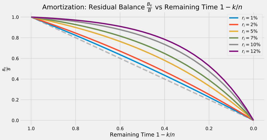
Figure 9. Amortization: residual balance \(B_k/B\) vs. residual time \(1-k/n\) for different interest rates. The dashed line is the \(r_i = 0\%\) case, where we have \(B_k = B(1-k/n)\).
| $1-\frac{k}{n}$ | $1\%$ | $2\%$ | $5\%$ | $7\%$ | $10\%$ | $12\%$ |
|---|---|---|---|---|---|---|
| 1.00 | 1.00 | 1.00 | 1.00 | 1.00 | 1.00 | 1.00 |
| 0.90 | 0.91 | 0.92 | 0.95 | 0.97 | 0.98 | 0.99 |
| 0.80 | 0.82 | 0.84 | 0.90 | 0.93 | 0.96 | 0.97 |
| 0.70 | 0.73 | 0.76 | 0.84 | 0.88 | 0.92 | 0.95 |
| 0.60 | 0.64 | 0.67 | 0.76 | 0.82 | 0.88 | 0.91 |
| 0.50 | 0.54 | 0.57 | 0.68 | 0.74 | 0.82 | 0.86 |
| 0.40 | 0.44 | 0.47 | 0.58 | 0.65 | 0.74 | 0.78 |
| 0.30 | 0.33 | 0.37 | 0.47 | 0.53 | 0.62 | 0.68 |
| 0.20 | 0.22 | 0.25 | 0.33 | 0.39 | 0.47 | 0.53 |
| 0.10 | 0.11 | 0.13 | 0.18 | 0.22 | 0.27 | 0.31 |
| 0.00 | 0.00 | 0.00 | 0.00 | 0.00 | 0.00 | 0.00 |
Partial Interest
The bulging from the amortization from above is a key factor to be considered when refinancing. Let us first derive a formula for the interest paid until time \(k\). While not strictly necessary it is helpful to understand the effects a little better.Until time \(k\) we make \(M k\) payments and the residual balance is \(B_k\). Thus we have:
\[\tag{interestPaid} \begin{align*} I_k &= M k - (B - B_k) \\ &= \frac{B}{n} E(r_i,n) k - (B - B_k) \\ &= \frac{B}{n} E(r_i,n) k - B + B \left(1-\frac{k}{n}\right) \frac{E(r_i,n)}{E(r_i,n-k)} \\ &= B \left( \frac{k}{n} E(r_i,n) + \left(1-\frac{k}{n}\right) \frac{E(r_i,n)}{E(r_i,n-k)} - 1 \right), \end{align*}\]Cleaning this up gets us a particular expansion factor \(E_k(r_i,n)\) defined as:
\[\tag{expansionFactorK} \begin{align*} E_k(r_i,n) & \doteq \underbrace{\frac{k}{n} E(r_i,n)}_{\text{proportional expansion}} + \underbrace{\left(1-\frac{k}{n}\right) \frac{E(r_i,n)}{E(r_i,n-k)}}_{\text{correction due to bulging}}, \end{align*}\]which is a convex combination of the expansion factor \(E(r_i,n)\) and a correction term \(\frac{E(r_i,n)}{E(r_i,n-k)}\). With this we can rewrite the above as
\[\tag{totalPaidToK} P + I_k = B + I_k = B E_k(r_i,n).\]and hence the interest paid up to time \(k\) is
\[\tag{interestPaidToK} I_k = B \left( E_k(r_i,n) - 1 \right).\]Below we plot \(E_k(r_i,n)\) for different interest rates and times \(k\) (with \(n=30\) but this is not important). We used our approximation \(\tilde E(r_i,n)\) for the actual computations below; the error is negligible and hence we write \(E_k(r_i,n) = \tilde E(r_i,n_k)\) here.
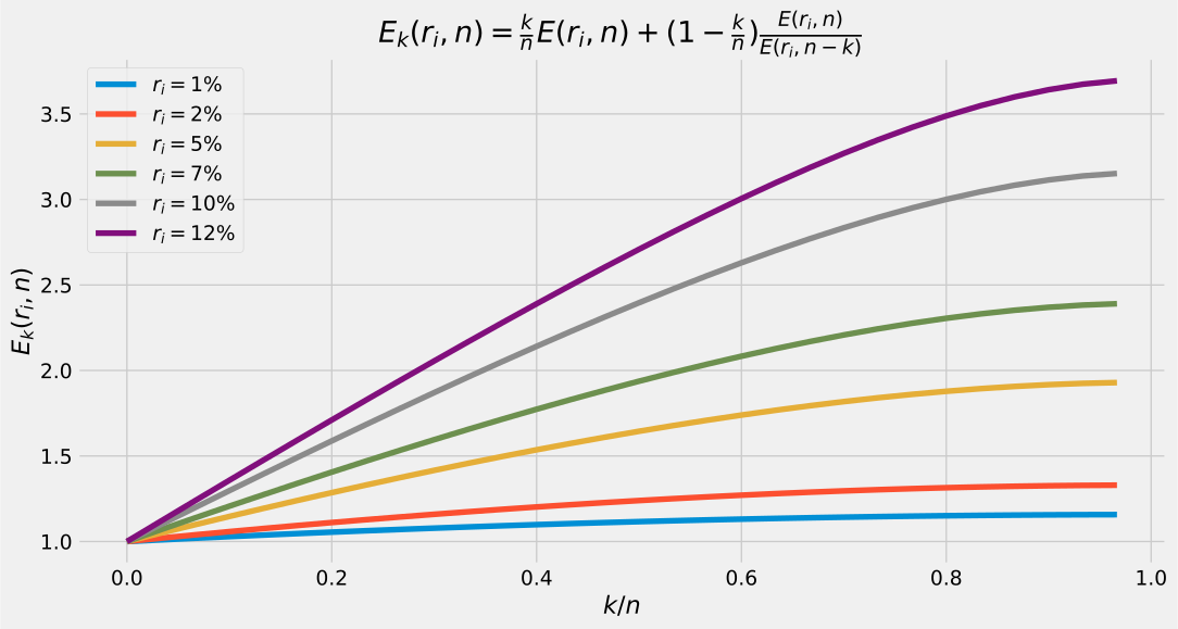
Figure 10. Expansion factor \(E_k(r_i,n)\) up to time \(k\).
If we compare \(E_k(r_i,n)\) to \(k/n E(r_i,n)\), which is the proportional attribution of the expansion over the duration of the mortgage, we see that the bulk of the interest payments happens early on (see Figure below).
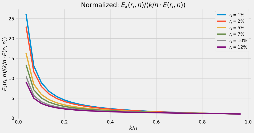
Figure 11. Expansion factor \(E_k(r_i,n)\) up to time \(k\) normalized by \(k/n E(r_i,n)\), which would be the proportional attribution of the expansion over the duration of the mortgage.
Refinancing
Let us now turn our attention to actual refinancing. The basic setup is that we make payments \(M\) up to time \(k\) and then we refinance the residual balance \(B_k\) at a new interest rate \(r_j\) but typically the duration resets to \(n\). If it would not reset and the interest rate would stay the same there is nothing to be gained or lost from refinancing. However, the interest rate is typically lower but the durations resets so that it is a priori not clear whether we can potentially save money.
Using \(M = \frac{B}{n} E(r_i,n)\) we can write the total payments as:
\[\begin{align*} M k + B_k E(r_j,n) & = B \frac{k}{n} E(r_i,n) + B_k E(r_j,n) \\ & = B \frac{k}{n} E(r_i,n) + B \left(1- \frac{k}{n}\right) \frac{E(r_i,n)}{E(r_i,n-k)} E(r_j,n) \\ & = B E(r_i,n) \underbrace{\left( \frac{k}{n} + \left(1- \frac{k}{n}\right) \frac{E(r_j,n)}{E(r_i,n-k)} \right)}_{\text{refinancing factor}} \end{align*}\]Example.
We consider a simple scenario to demonstrate this effect. Suppose we have a $30$-year mortgage at $5\%$ interest rate that we pay off completely. Then we have:
\[E(5\%, 30) \approx 1.93,\]i.e., we pay roughly \(0.93\) interest on top of every dollar. Now let us consider the scenario where we refinance after \(15\) years. We can either refinance at the same interest rate of \(5\%\) or at a lower interest rate of \(3\%\):
\[15 M + B_{15} E(0.03,30) \approx 2.00,\]i.e., it is more expensive. This effect can be nicely seen below in the two figures.
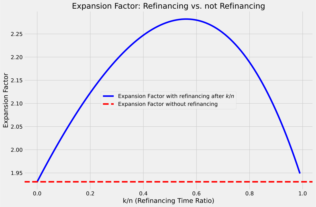
Figure 12. 30-year mortgage at \(5\%\) interest rate refinanced at \(5\%\) interest rate. No refinancing in (red) and refinancing in (blue). In this case it never makes sense to refinance.
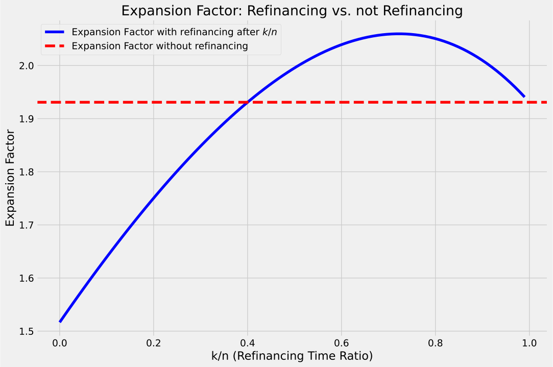
Figure 13. 30-year mortgage at \(5\%\) interest rate refinanced at \(3\%\) interest rate. No refinancing in (red) and refinancing in (blue). In this case it makes sense to refinance on the early time of the mortgage until roughly the \(40\%\) mark.
Early Repayment
Another interesting effect is early repayment. Suppose we have a mortgage at \(r_i\) for \(n\) years and we “suddenly” happen to find another chunk of money to do a one-shot payment right at the beginning to pay off some of the principal but keep the mortgage alive as is, in particular the recurring payment \(M\) does not change. What is the net effect on this?
The math for this is relatively simple given what we have computed so far. We have \(M = \frac{B}{n} E(r_i,n)\). Doing our one-shot payment of a fraction $\alpha$ leads to a new principal $(1-\alpha)B$. Since the recurring payment \(M\) has not changed and the interest rate stays the same this effectively amounts to a modified duration \(\tilde n\). To simplify the math we use \(\tilde E\) right away. We have the identity:
\[\begin{align*} & \frac{B}{n} \tilde E(r_i,n) = M = \frac{(1-\alpha)B}{\tilde n} \tilde E(r_i,\tilde n) \\ \Rightarrow\quad & \frac{B}{n} \frac{r_i n}{1-e^{-r_i n}} = \frac{(1-\alpha)B}{\tilde n} \frac{r_i \tilde n}{1-e^{-r_i \tilde n}} \\ \Rightarrow\quad & \frac{1}{1-e^{-r_i n}} = (1-\alpha) \frac{1}{1-e^{-r_i \tilde n}} \\ \Rightarrow\quad & 1-e^{-r_i \tilde n} = (1-\alpha) (1-e^{-r_i n}) \\ \Rightarrow\quad & 1 - (1-\alpha) (1-e^{-r_i n}) = e^{-r_i \tilde n} \\ \Rightarrow\quad & \tilde n = - \frac{\log(1 - (1-\alpha) (1-e^{-r_i n}))}{r_i} = - \frac{\log(\alpha+ (1-\alpha) e^{-r_i n})}{r_i}, \end{align*}\]and we define the modified duration \(\tilde n\) as:
\[\tag{modifiedDuration} \tilde n \doteq - \frac{\log(\alpha+ (1-\alpha) e^{-r_i n})}{r_i}.\]In the figure below we plot the modified duration \(\tilde n\) for different values of \(\alpha\) and \(r_i\) (with \(n=30\)).
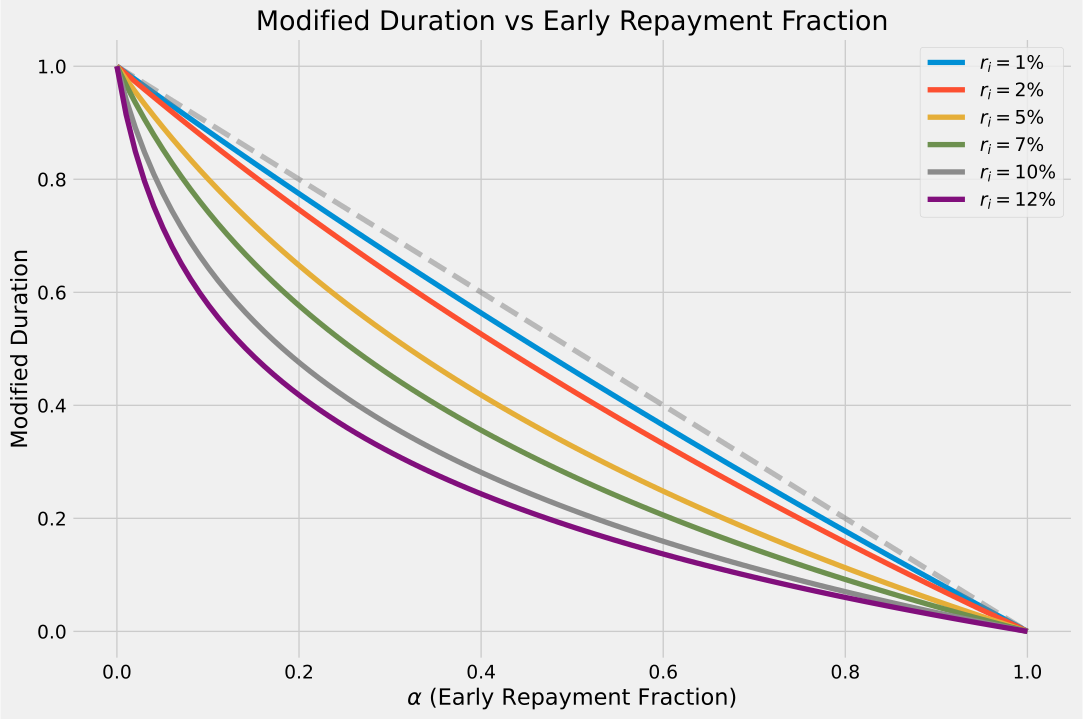
Figure 14. Modified duration \(\tilde n\) for different values of \(\alpha\) and \(r_i\) (with \(n=30\)). At high interest rates an early repayment of \(20\%\) can reduce the effective duration down to roughly \(40\%\) of the original duration!
What what does this effectively in terms of expansion factors and interest savings? For this below the next two figures show the expansion factor \(E(r_i,\tilde n)\) as a function of \(\alpha\) for different interest rates \(r_i\) (with \(n=30\)) (Figure 15) and the normalized expansion factor \(E(r_i,\tilde n)/E(r_i,n)\) (Figure 16); the latter measures the fraction of the original expansion factor (and hence interest cost) that is left.
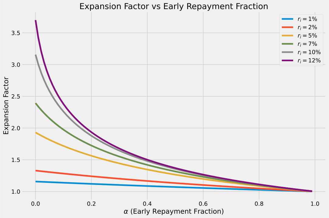
Figure 15. Expansion factor \(E(r_i,\tilde n)\) for different values of \(\alpha\) and \(r_i\) (with \(n=30\)).
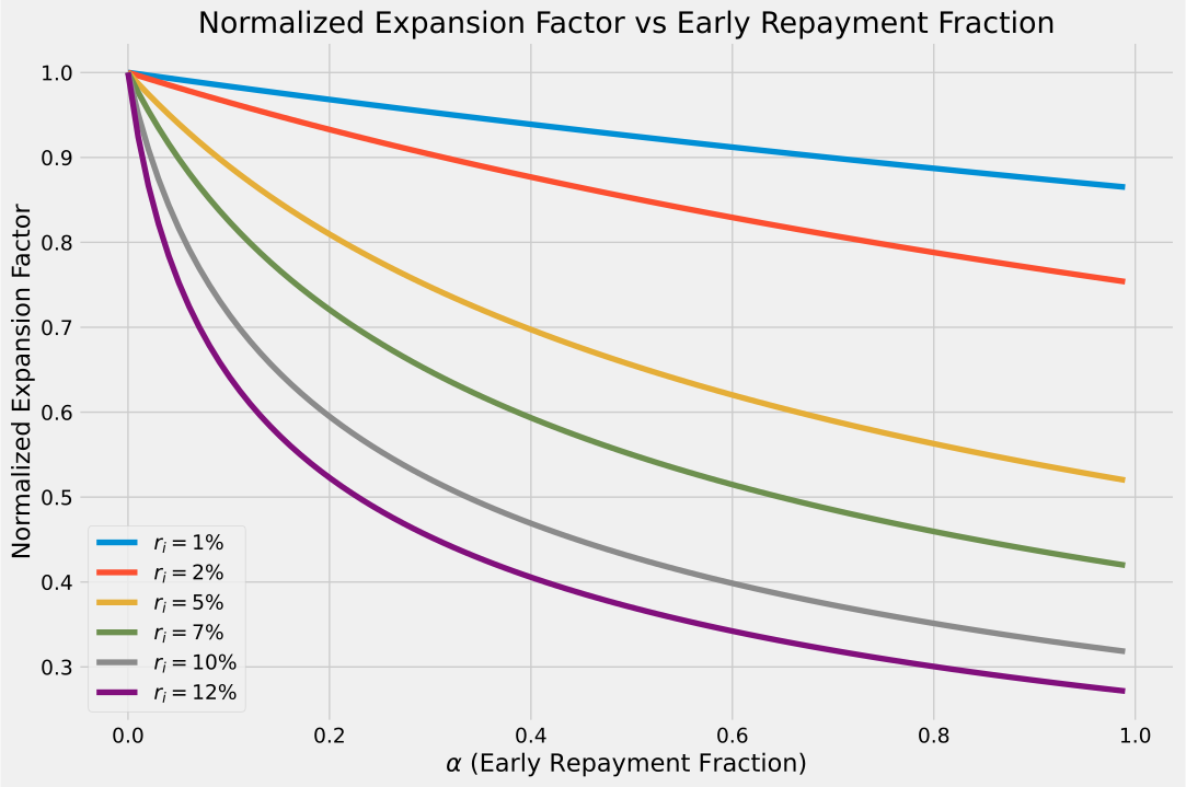
Figure 16. Normalized expansion factor \(E(r_i,\tilde n)/E(r_i,n)\) for different values of \(\alpha\) and \(r_i\) (with \(n=30\)).
Finally, so when does it make sense to do an early repayment? The following figure shows the difference in interest cost between the original mortgage and the partially repaid mortgage, i.e., \(E(r_i,n) - E(r_i,\tilde n)\) as a function of \(\alpha\) for different interest rates \(r_i\) (with \(n=30\)).
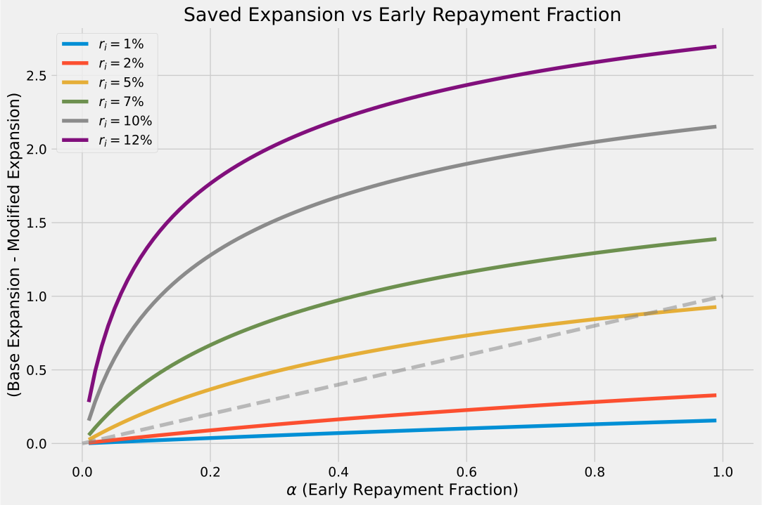
Figure 17. Interest cost difference \(E(r_i,n) - E(r_i,\tilde n)\) as a function of \(\alpha\) for different interest rates \(r_i\) (with \(n=30\)). The dashed line is the economic frontier, i.e., if we repay \(\alpha\) early then the cost better drop by at least that much, i.e., \(E(r_i,n) - E(r_i,\tilde n) \geq \alpha\). For everything above that line early repayment makes sense; for everything below it does not.
Rent vs. Buy (rough estimation)
This brings us to the final part of our mortgage journey: the rent vs. buy decision. There are tons of approaches to look at this problem, cost-based, total unrecoverable costs, etc. I usually used total unrecoverable costs however while “actuarial” in some sense it is too fine-grained on the one hand and on the other hand it does not properly account for opportunity costs. Therefore this time around I want to take a different approach, where we compare two “portfolios”. The first one is our null-portfolio, i.e., we do not buy a house and instead rent it and where we invest the money in the market at appropriate returns after inflation. The second portfolio is the buy-portfolio, i.e., where we buy a house and pay off the mortgage. We then compare the two portfolios in terms of total total value over time. We subtract from all rates the risk-free rate \(r_f\) to account for inflation, so that the reported value is roughly the net present value.
Cost terms.
- \(M\): monthly payment (for simplicity we assume that it contains all costs, i.e., maintenance, property tax, etc.)
- \(R\): monthly rent
- \(A\): acquisition costs (including closing costs)
- \(P\): principal
Rates.
- \(r_e\): monthly return on equity
- \(r_r\): monthly return on real estate
- \(r_f\): monthly risk-free or inflation rate (we assume that the two are the same)
- \(r_i\): monthly interest rate
Null-portfolio. In this case we have after time \(k\) the following portfolio value:
\[\begin{align*} & \underbrace{- R \sum_{m=1}^k (1+ r_f)^m}_{\text{rent}} + \underbrace{\left(M - R\right) \sum_{m=1}^k (1+ r_e)^m}_{\text{investment}} \\ =\quad & - R \left(\frac{(1+r_f)^{k+1}-1}{r_f} -1 \right) + \left(M - R\right) \left( \frac{(1+ r_e)^{k+1} - 1}{r_e} - 1 \right). \end{align*}\]Note that we assume that the rent is inflation-adjusted. Moreover, the term \(M-R\) does not include the increase in rent due to inflation, the rough reasoning being that it is reasonable to assume that \(M\) is also growing with inflation, so that the delta roughly remains the same. This is a simplifcation making the rent-case a little more favorable; without such an assumption, the \(R\) might “inflate away” the \(M\) (if it is not adjusted) and no investment gains are to be had.
Buy-portfolio. In this case we have after time \(k\) the following portfolio value:
\[\begin{align*} & - \underbrace{M k}_{\text{mortgage payments}} - \underbrace{A (1+r_e)^k}_{\text{acquistion}} + \underbrace{P (1+r_r)^k}_{\text{real estate gain}} - \underbrace{B_k}_{\text{residual balance}} \\ =\quad & - M k - A (1+r_e)^k + P (1+r_r)^k - P \frac{1-e^{-r_i(n-k)}}{1 - e^{-r_i n}} \end{align*}\]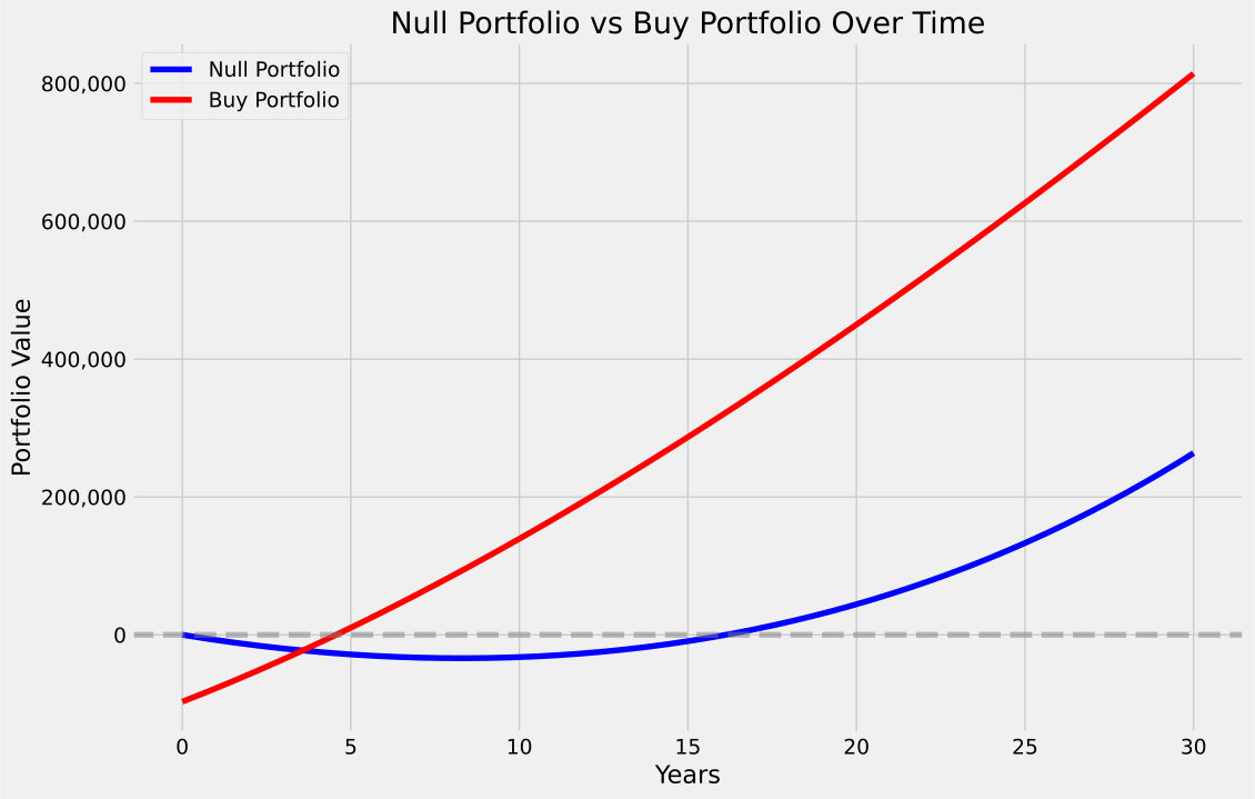
Figure 18. Buy-portfolio value vs. time for different interest rates \(r_i\) (with \(n=30\)).
Note. A purely financial analysis might not be sufficient as there are exogeneous risk factors, e.g., unexpected changes in the economy, unexpected changes in the real estate market, etc. that are not properly priced for. Thus the above can only serve as a rough guide augmenting the decision making process.
References
[P] Pokutta, Sebastian. “Restarting Algorithms: Sometimes there is Free Lunch”. Proceedings of CPAIOR. 2020. pdf
Changelog
- 2024-12-27: Added section on mortgages, mortrage approximation, and losses due to cap gains.
Comments