CINDy: Conditional gradient-based Identification of Non-linear Dynamics
TL;DR: This is an informal summary of our recent paper CINDy: Conditional gradient-based Identification of Non-linear Dynamics – Noise-robust recovery by Alejandro Carderera, Sebastian Pokutta, Christof Schütte and Martin Weiser where we propose the use of a Conditional Gradient algorithm (more concretely the Blended Conditional Gradients [BPTW] algorithm) for the sparse recovery of a dynamic. In the presence of noise, the proposed algorithm presents superior sparsity-inducing properties, while ensuring a higher recovery accuracy, compared to other existing methods in the literature, most notably the popular SINDy [BPK] algorithm, based on a sequentially-thresholded least-squares approach.
Written by Alejandro Carderera.
What is the paper about and why you might care
A large number of humankind’s scientific breakthroughs have been fueled by our ability to describe natural phenomena in terms of differential equations. These equations give us a condensed representation of the underlying dynamics and have helped build our understanding of natural phenomena in many scientific disciplines.
The modern age of Machine Learning and Big Data has heralded an age of data-driven models, in which the phenomena we explain are described in terms of statistical relationships and data. Given sufficient data, we are able to train neural networks to classify or to predict, with high accuracy, without the underlying model having any apparent knowledge of how the data was generated or its structure. This makes the task of classifying or predicting, on out-of-sample data a particularly challenging task. Due to this, there has been a recent surge in interest in recovering the differential equations with which the data, often coming from a physical system, have been generated. This enables us to better understand how the data is generated and to better predict on out-of-sample data.
Learning sparse dynamics
Many physical systems can be described in terms of ordinary differential equations of the form $\dot{x}(t) = F\left(x(t)\right)$, where $x(t) \in \mathbb{R}^d$ denotes the state of the system at time $t$ and $F: \mathbb{R}^d \rightarrow \mathbb{R}^d$ can usually be expressed as a linear combination of simpler ansatz functions $\psi_i: \mathbb{R}^d \rightarrow \mathbb{R}$ belonging to a dictionary \(\mathcal{D} = \left\{\psi_i \mid 1 \leq i \leq n \right\}\). This allows us to express the dynamic followed by the system as $\dot{x}(t) = F\left(x(t)\right) = \Xi^T \bm{\psi}(x(t))$ where $\Xi \in \mathbb{R}^{n \times d}$ is a – typically sparse – matrix $\Xi = \left[\xi_1, \cdots, \xi_d \right]$ formed by column vectors $i_i \in \mathbb{R}^n$ for $1 \leq i \leq n$ and $\bm{\psi}(x(t)) = \left[ \psi_1(x(t)), \cdots, \psi_n(x(t)) \right]^T \in \mathbb{R}^{n}$. We can therefore write:
\[\dot{x}(t) = \begin{bmatrix} \rule{.5ex}{2.5ex}{0.5pt} & \xi_1 & \rule{.5ex}{2.5ex}{0.5pt}\\ & \vdots & \\ \rule{.5ex}{2.5ex}{0.5pt} & \xi_d & \rule{.5ex}{2.5ex}{0.5pt} \end{bmatrix} \begin{bmatrix} \psi_1(x(t)) \\ \vdots \\ \psi_n(x(t)) \end{bmatrix}.\]In the absence of noise, if we are given a series of data points from the physical system \(\left\{ x(t_i), \dot{x}(t_i) \right\}_{i=1}^m\), then we know that:
\[\begin{bmatrix} \rule{-1ex}{0.5pt}{2.5ex} & & \rule{-1ex}{0.5pt}{2.5ex}\\ \dot{x}(t_1) & \cdots & \dot{x}(t_m)\\ \rule{-1ex}{0.5pt}{2.5ex} & & \rule{-1ex}{0.5pt}{2.5ex} \end{bmatrix} = \begin{bmatrix} \rule{.5ex}{2.5ex}{0.5pt} & \xi_1 & \rule{.5ex}{2.5ex}{0.5pt}\\ & \vdots & \\ \rule{.5ex}{2.5ex}{0.5pt} & \xi_d & \rule{.5ex}{2.5ex}{0.5pt} \end{bmatrix} \begin{bmatrix} \rule{-1ex}{0.5pt}{2.5ex} & & \rule{-1ex}{0.5pt}{2.5ex}\\ \bm{\psi}\left(x(t_1)\right) & \cdots & \bm{\psi}\left(x(t_m)\right)\\ \rule{-1ex}{0.5pt}{2.5ex} & & \rule{-1ex}{0.5pt}{2.5ex} \end{bmatrix}.\]If we collect the data in matrices $\dot{X} = \left[ \dot{x}(t_1),\cdots, \dot{x}(t_m)\right] \in\mathbb{R}^{d\times m}$, $\Psi\left(X\right) = \left[ \bm{\psi}(x(t_1)),\cdots, \bm{\psi}(x(t_m))\right]\in\mathbb{R}^{n\times m}$, we can try to recover the underlying sparse dynamic by attempting to solve:
\[\min\limits_{\dot{X} = \Omega^T \Psi(X)} \left\| \Omega\right\|_0.\]Unfortunately, the aforementioned problem is a notoriously difficult NP-hard combinatorial problems, due to the presence of the $\ell_0$ norm in the objective function of the problem. Moreover, if the data points are contaminated by noise, leading to noisy matrices $\dot{Y}$ and $\Psi(Y)$, depending on the expressive power of the basis functions $\psi_i$ for $1\leq i \leq n$, it may not even be possible (or desirable) to satisfy $\dot{Y} = \Omega^T \Psi(Y)$ for any $\Omega \in \mathbb{R}^{n\times d}$. Thus one can attempt to convexify the problem, substituting the $\ell_0$ norm (which is technically not a norm) for the $\ell_1$ norm. That is, solve for a suitably chosen $\epsilon >0$
\[\tag{BPD} \min\limits_{ \left\|\dot{Y} - \Omega^T \Psi(X) \right\|^2_F \leq \epsilon } \left\|\Omega\right\|_{1,1} \label{eq:l1_minimization_noisy2}\]This leads us to a formulation, known as Basis Pursuit Denoising (BPD) [CDS], which was initially developed by the signal processing community, and is intimately tied to the Least Absolute Shrinkage and Selection Operator (LASSO) regression formulation [T], developed in the statistics community. The latter formulation, which we will use for this problem, takes the form:
\[\tag{LASSO} \min\limits_{ \left\|\Omega\right\|_{1,1} \leq \alpha} \left\|\dot{Y} - \Omega^T \Psi(X) \right\|^2_F\]Both problems shown in (BPD) and (LASSO) have a convex objective function and a convex feasible region, which allows us to use the powerful tools and guarantees of convex optimization. Moreover, there is a significant body of theoretical literature, both from the statistics and the signal processing community, on the conditions for which we can successfully recover the support of $\Xi$ (see e.g., [W]), the uniqueness of the LASSO solutions (see e.g., [T2]), or the robust reconstruction of phenomena from incomplete data (see e.g., [CRT]), to name but a few results.
Incorporating structure into the learning problem
Conservation laws are a fundamental pillar of our understanding of physical systems. Imposing these laws through (symmetry) constraints in our sparse regression problem can potentially lead to better generalization performance under noise, reduced sample complexity, and to learned dynamics that are consistent with the symmetries present in the real world. In particular, there are two large classes of structural constraints that can be easily encoded into our learning problem as linear constraints:
- Conservation properties: We often observe in dynamical systems that certain relations hold between the elements of $\dot{x}(t)$. Such is the case in chemical reaction dynamics, where if we denote the rate of change of the $i$-th species by $\dot{x}_i(t)$, we might observe relations of the form $a_j\dot{x}_j(t) + a_k\dot{x}_k(t) = 0$ due to mass conservation, which relate the $j$-th and $k$-th species being studied.
- Symmetry between variables: One of the key assumptions used in many-particle quantum systems is the fact the particles being studied are indistinguishable. And so it makes sense to assume that the effect that the $i$-th particle exerts on the $j$-th particle is the same as the effect that the $j$-th particle exerts on the $i$-th particle. The same can be said in classical mechanics for a collection of identical masses, where each mass is connected to all the other masses through identical springs. These restrictions can also be added to our learning problem as linear constraints.
If we were to add $L$ additional linear constraints to the problem in (LASSO) to reflect the underlying structure of the dynamical system through symmetry and conservation, we would arrive at a polytope $\mathcal{P}$ of the form
\[\mathcal{P} = \left\{ \Omega \in \mathbb{R}^{n \times d} \mid \left\|\Omega\right\|_{1,1} \leq \tau, \text{trace}( A_l^T \Omega ) \leq b_l, 1 \leq l \leq L \right\},\]for an appropriately chosen $A_l$ and $b_l$.
Blended Conditional Gradients
The problem is that in the presence of noise many learning approaches see their sparsity-inducing properties quickly degrade, producing dense dynamics that are far from the true dynamic, this is often what happens with the sequentially-thresholded least-squares algorithm in [BPK], which underlies SINDy. Ideally, we want to look for learning algorithms that are somewhat robust to the presense of noise. Moreover, it would also be advantageous if we could easily incorporate structural linear constraints into the learning problem, as described in the previous section, to lead to learned dynamics that are consistent with the true dynamic.
For the recovery of sparse dynamics from data, one of the most interesting algorithms in terms of sparsity is the Fully-Corrective Conditional Gradient algorithm. This algorithm picks up a vertex $V_k$ from the polytope $\mathcal{P}$ using a linear optimization oracle, and reoptimizes over the convex hull of $\mathcal{S}_{k} \bigcup V_k$, which is the union of the vertices picked up in previous iterations, and the new vertex $V_k$. One of the key advantages of requiring a linear optimization oracle, instead of a projection oracle, to solve the optimization problem is that for general polyhedral constraints there are efficient algorithms to solve linear optimization problems, whereas solving a quadratic problem to compute a projection can be too computationally expensive.
Fully-Corrective Conditional Gradient (CG) algorithm applied to (LASSO)
Input: Initial point $\Omega_1 \in \mathcal{P}$
Output: Point $\Omega_{K+1} \in \mathcal{P}$
\(\mathcal{S}_{1} \leftarrow \emptyset\)
For \(k = 1, \dots, K\) do:
$\quad \nabla f \left( \Omega_k \right) \leftarrow 2 \Psi(Y) \left(\dot{Y} - \Omega_k^T\Psi(Y) \right)^T$
$\quad V_k \leftarrow \min\limits_{\Omega \in \mathcal{P}} \text{trace}\left(\Omega^T\nabla f \left( \Omega_k \right) \right)$
\(\quad \mathcal{S}_{k+1}\leftarrow \mathcal{S}_{k} \bigcup V_k\)
\(\quad \Omega_{k+1} \leftarrow \min\limits_{\Omega \in \text{conv}\left( \mathcal{S}_{k+1} \right) } \left\|\dot{Y} - \Omega^T \Psi(Y)\right\|^2_F\)
End For
To get a better feel of the sparsity inducing properties of the FCFW algorithm, if we assume that the starting point $\Omega_1$ is a vertex of the polytope, then we know that the iterate $\Omega_k$ can be expressed as a convex combination of at most $k$ vertices of $\mathcal{P}$. This is due to the fact that the algorithm can pick up no more than one vertex per iteration. Note that if $\mathcal{P}$ were the $\ell_1$ ball without any additional constraints, the FCFW algorithm picks up at most one basis function in the $k$-th iteration, as $V_k^T \bm{\psi}(x(t)) = \pm \tau \psi_i(x(t)$ for some $1\leq i\leq n$. This means that if we use the Frank-Wolfe algorithm to solve a problem over the $\ell_1$ ball, we encourage sparsity not only through the regularization provided by the $\ell_1$ ball, but also through the specific nature of the Frank-Wolfe algorithm independently of the size of the feasible region. In practice, when using, e.g., early termination due to some stopping criterion, this results in the Frank-Wolfe algorithm producing sparser solutions than projection-based algorithms (such as projected gradient descent, which typically uses dense updates).
Reoptimizing over the union of vertices picked up can be an expensive operation, especially if there are many such vertices. An alternative is to compute these reoptimizations to $\varepsilon_k$-optimality at iteration $k$. However, this leads to the question: How should we choose $\varepsilon_k$ at each iteration $k$, if we want to find an $\varepsilon$-optimal solution to (LASSO)? Computing a solution to the problem to accuracy $\varepsilon_k = \varepsilon$ at each iteration might be way too computationally expensive. Conceptually, we need relatively inaccurate solutions for early iterations where \(\Omega^\esx \notin \text{conv} \left(\mathcal{S}_{k+1}\right)\), requiring only accurate solutions when \(\Omega^\esx \in \text{conv} \left(\mathcal{S}_{k+1}\right)\). At the same time we do not know whether we have found \(\mathcal{S}_{k+1}\) so that \(\Omega^\esx \in \text{conv} \left(\mathcal{S}_{k+1}\right)\).
The rationale behind the Blended Conditional Gradient (BCG) algorithm [BPTW] is to provide an explicit value of the accuracy $\varepsilon_k$ needed at each iteration starting with rather large \(\varepsilon_k\) in early iterations and progressively getting more accurate when approaching the optimal solution; the process is controlled by an optimality gap measure. In some sense one might think of BCG as a practical version of FCCG with stronger convergence guarantees and much faster real-world performance.
CINDy: Blended Conditional Gradient (BCG) algorithm variant applied to (LASSO) problem
Input: Initial point $\Omega_0 \in \mathcal{P}$
Output: Point $\Omega_{K+1} \in \mathcal{P}$
\(\Omega_1 \leftarrow \text{argmin}_{\Omega \in \mathcal{P}} \text{trace}\left(\Omega^T\nabla f \left( \Omega_0 \right) \right)\)
\(\Phi \leftarrow \text{trace} \left( \left( \Omega_0 - \Omega_1\right)^T \nabla f(\Omega_0)\right)/2\)
\(\mathcal{S}_{1} \leftarrow \left\{ \Omega_1 \right\}\)
For \(k = 1, \dots, K\) do:
\(\quad\) Find $\Omega_{k+1} \in \operatorname{conv}(\mathcal{S}_{k})$ such that \(\max_{\Omega \in \mathcal{P}} \text{trace}\left((\Omega_{k+1} -\Omega )^T\nabla f \left( \Omega_{k+1} \right) \right) \leq \Phi\)
\(\quad V_{k+1} \leftarrow \text{argmin}_{\Omega \in \mathcal{P}} \text{trace}\left(\Omega^T\nabla f \left( \Omega_{k+1} \right) \right)\)
\(\quad\) If \(\left( \text{trace}\left( \left( \Omega_{k+1} -V_{k+1}\right)^T \nabla f(\Omega_{k+1})\right) \leq \Phi \right)\)
\(\quad\quad \Phi \leftarrow \text{trace}\left( \left( \Omega_{k+1} -V_{k+1}\right)^T \nabla f(\Omega_{k+1})\right)/2\)
\(\quad\quad \mathcal{S}_{k+1} \leftarrow \mathcal{S}_k\)
\(\quad\quad \Omega_{k+1} \leftarrow \Omega_k\)
\(\quad\) Else
\(\quad\quad\mathcal{S}_{k+1} \leftarrow \mathcal{S}_k \bigcup V_{k+1}\)
\(\quad\quad D_k \leftarrow V_{k + 1} - \Omega_k\)
\(\quad\quad \gamma_k \leftarrow \min\left\{-\frac{1}{2}\text{trace} \left( D_k^T \nabla f \left(
\Omega_k \right) \right)/ \left\| D_k^T
\Psi(Y)\right\|_F^2,1\right\}\)
\(\quad\quad \Omega_{k+1} \leftarrow \Omega_k + \gamma_k D_k\)
\(\quad\) End If
End For
As we will show numerically in the next section, the CINDy algorithm not only produces sparser solutions to the learning problem, it also exhibits a higher robustness with respect to noise than other existing approaches. This is in keeping with the law of parsimony (also called Occam’s Razor), which states that the simplest explanation, in our case the sparsest, is usually the right one (or close to the right one!).
Numerical experiments
We benchmark the CINDy algorithm applied to the LASSO sparse recovery formulations with the following algorithms. Our main benchmark here is the SINDy algorithm, however we included two more popular optimization methods for further comparison, namely, the Interior-Point Methods in CVXOPT [ADLVSNW], and the FISTA algorithm.
We use CINDy (c) and CINDy to refer to the results achieved by the CINDy algorithm with and without the additional structural constraints arising e.g., from conservation laws. Likewise, we use IPM (c) and IPM to refer to the results achieved by the IPM algorithm with and without additional constraints. We have not added structural constraints to the formulation in the SINDy algorithm, as there is no straightforward way to include constraints in the original implementation, or the FISTA algorithm, as we would need to compute non-trivial proximal/projection operators, making the algorithm computationally too expensive.
To benchmark the algorithms we use two different metrics, the recovery error defined as \(\mathcal{E}_{R} = \norm{\Omega - \Xi}_F\) and the number of extraneous terms defined as \(\mathcal{S}_E = \abs {\left\{ \Omega_{i,j} \mid \Omega_{i,j} \neq 0, \Xi_{i,j} = 0, 1 \leq i \leq d \in, 1 \leq j \leq n \right\}}\), i.e., those terms that do not belong to the dynamic.
Fermi-Pasta-Ulam-Tsingou model
The Fermi-Pasta-Ulam-Tsingou model describes a one-dimensional system of $d$ identical particles, where neighboring particles are connected with springs, subject to a nonlinear forcing term [FPUT]. This computational model was used at Los Alamos to study the behaviour of complex physical systems over long time periods. The equations of motion that govern the particles, when subjected to cubic forcing terms is given by \(\ddot{x}_i = \left(x_{i+1} - 2 x_i + x_{i-1} \right) + \beta \left[ \left( x_{i+1} - x_i \right)^3 - \left( x_{i} - x_{i-1} \right)^3 \right],\) where $1 \leq i \leq d$ and $x_{i}$ refers to the displacement of the $i$-th particle with respect to its equilibrium position. The exact dynamic $\Xi$ can be expressed using a dictionary of monomials of degree up to three.
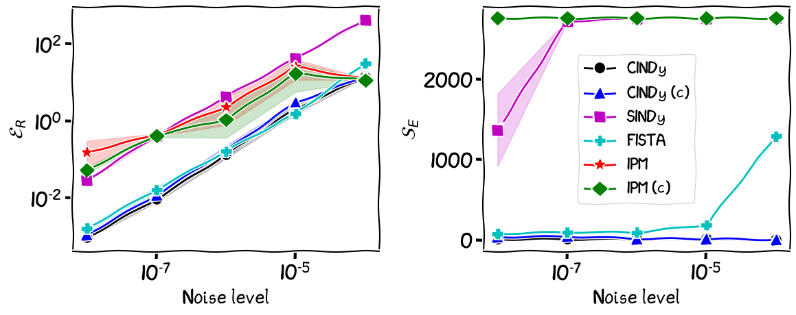
Figure 1. Sparse recovery of the Fermi-Pasta-Ulam-Tsingou dynamic with $d = 10$
As we can see in the images, there is a large difference between the CINDy and FISTA algorithms, and the remaining algorithms, with the former algorithms being up to two orders of magnitude more accurate in terms of $\mathcal{E}_R$, while algo being much sparser, as seen in the image that depicts $\mathcal{S}_E$.
However, what does this difference in recovery error translate to? We can see the difference in accuracy between the different learned dynamics by simulating forward in time the dynamic learned by the CINDy algorithm and the SINDy algorithm, and comparing that to the evolution of the true dynamic. The results in the next image show this comparison for different times for the dynamics learnt by the two algorithms with a noise level of $10^{-4}$ for the example of dimensionality $d = 10$. In keeping with the physical nature of the problem, we present the ten dimensional phenomenon as a series of oscillators suffering a displacement on the vertical y-axis, in a similar fashion as was done in the original paper SINDy paper [BPK]. Note that we have added to the images the two extremal particles on the left and right that do not oscillate. While CINDy’s trajectory matches that of the real dynamic up to very small error—it is also much smoother in time—the learned dynamic of SINDy is very far away from the true dynamics not even recovering essential features of the oscillation; the large number of additional terms deform the essential structure of the dynamic.
Figure 2. Fermi-Pasta-Ulam-Tsingou dynamic: Simulation of learned trajectories vs true trajectory.
Kuramoto model
The Kuramoto model [K] describes a large collection of $d$ weakly coupled identical oscillators, that differ in their natural frequency $\omega_i$. This dynamic is often used to describe synchronization phenomena in physics. If we denote by $x_i$ the angular displacement of the $i$-th oscillator, then the governing equation with external forcing can be written as: \(\dot{x}_i = \omega_i + \frac{K}{d}\sum_{j=1}^d \left[\sin \left( x_j \right) \cos \left( x_i \right) - \cos \left( x_j \right) \sin \left( x_i \right) \right]+ h\sin \left( x_i\right),\) for $1 \leq i \leq d$, where $d$ is the number of oscillators (the dimensionality of the problem), $K$ is the coupling strength between the oscillators and $h$ is the external forcing parameter. The exact dynamic $\Xi$ can be expressed using a dictionary of basis functions formed by sine and cosine functions of $x_i$ for $1 \leq i \leq d$, and pairwise combinations of these functions, plus a constant term.
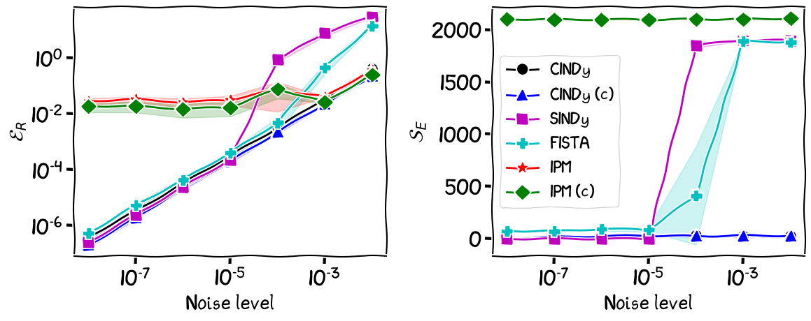
Figure 3. Sparse recovery of the Kuramoto dynamic with $d = 10$.
All algorithms except the IPM algorithms exhibit similar performance with respect to $\mathcal{E}_R$ and $\mathcal{S}_E$ up to a noise level of $10^{-5}$, however, the performance of the FISTA and SINDy algorithms degrade for noise levels above $10^{-5}$, producing solutions that are both dense (see $\mathcal{S}_E$), and are far away from the true dynamic (see $\mathcal{E}_R$). When we simulate the Kuramoto system from a given initial position, the algorithms have very different performances.
The next animation shows the results after simulating the dynamics learned by the CINDy and SINDy algorithm from the integral formulation for a Kuramoto model with $d = 10$ and a noise level of $10^{-3}$. In order to see more easily the differences between the algorithms and the position of the oscillators, we have placed the $i$-th oscillator at a radius of $i$, for $1 \leq i\leq d$. Note that the same coloring and markers are used as in the previous section to depict the trajectory followed by the exact dynamic, the dynamic learned with CINDy, and the dynamic learned with SINDy. As before while CINDy can reproduce the correct trajectory up to small error the trajectory of SINDy’s learned dynamic is rather far away from the real dynamic.
Figure 4. Kuramoto dynamic: Simulation of learned trajectories. Green is the true dynamic. Black is the dynamic learned via CINDy. Magenta is the dynamic learned via SINDy.
If we compare the CINDy and SINDy algorithms from the perspective of the sample efficiency, that is, the evolution of the error as we vary the number of training samples made available to the algorithm, and the noise levels, we can see that there is an additional benefit to the use of a CG-based algorithm for the recovery of the sparse dynamic and that inclusion of conversation laws can further improve sample efficiency and noise robustness.
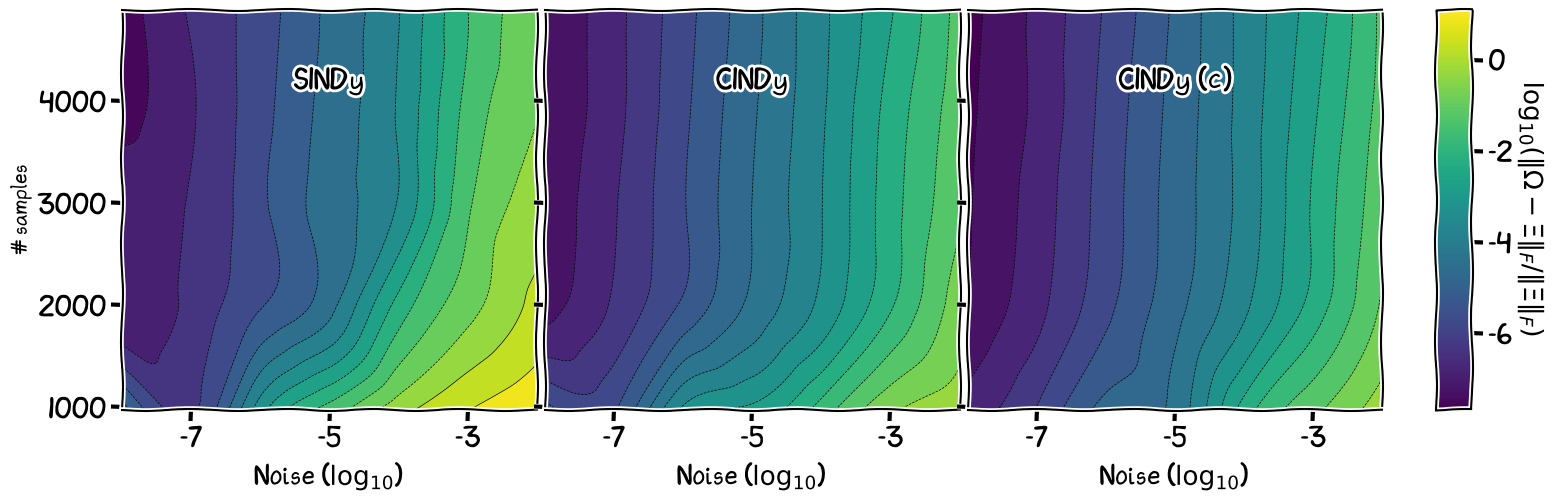
Figure 5. Kuramoto dynamic: Sample efficiency with $d = 5$.
If we focus for example on the bottom right corner for each of the images, we can see that the SINDy algorithm outputs dynamics with a lower accuracy in the low-training sample regime for higher noise levels, as compared to the CINDy algorithm.
Michaelis-Menten model
The Michaelis-Menten model [MM] is used to describe enzyme reaction kinetics. We focus on the following derivation, in which an enzyme E combines with a substrate S to form an intermediate product ES with a reaction rate $k_{f}$. This reaction is reversible, in the sense that the intermediate product ES can decompose into E and S, with a reaction rate $k_{r}$. This intermediate product ES can also proceed to form a product P, and regenerate the free enzyme E. This can be expressed as
\[S + E \rightleftharpoons E.S \to E + P.\]If we assume that the rate for a given reaction depends proportionately on the concentration of the reactants, and we denote the concentration of E, S, ES and P as $x_{\text{E}}$, $x_{\text{S}}$, $x_{\text{ES}}$ and $x_{\text{P}}$, respectively, we can express the dynamics of the chemical reaction as:
\[\begin{align*} \dot{x}_{\text{E}} &= -k_f x_{\text{E}} x_{\text{S}} + k_r x_{\text{ES}} + k_{\text{cat}} x_{\text{ES}} \\ \dot{x}_{\text{S}} &= -k_f x_{\text{E}} x_{\text{S}} + k_r x_{\text{ES}} \\ \dot{x}_{\text{ES}} &= k_f x_{\text{E}} x_{\text{S}} - k_r x_{\text{ES}} - k_{\text{cat}} x_{\text{ES}} \\ \dot{x}_{P} &= k_{\text{cat}} x_{\text{ES}}. \end{align*}\]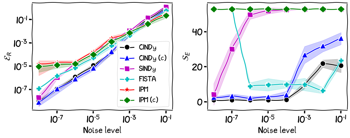
Figure 6. Sparse recovery of the Michaelis-Menten dynamic with $d = 4$. Left is recovery error in Frobenius norm. Right is number of extra terms picked up that do not belong to dynamic.
We can observe that for the lowest noise levels, the CINDy algorithm presents no advantage over the SINDy algorithm, however, as we crank up the noise levels, the performance of SINDy degrades, as the algorithm picks up more and more extra terms that are not present in the true dynamic. For low to moderately high noise levels the CINDy algorithm provides the best performance, with the lowest error in terms of $\mathcal{E}_R$, and the sparsest solutions in terms of $\mathcal{S}_E$. For very high noise levels, all the algorithms perform similarly in terms of $\mathcal{E}_R$, while CINDy’s recoveries are still significantly sparser than those of SINDy.
References
[BPK] Brunton, S.L., Proctor, J.L. , and Kutz, J.N. (2016) Discovering governing equations from data by sparse identification of nonlinear dynamical systems. In Proceedings of the national academy of sciences 113.15 : 3932-3937 pdf
[BPTW] Braun, G., Pokutta, S., Tu, D., & Wright, S. (2019). Blended conditonal gradients. In International Conference on Machine Learning (pp. 735-743). PMLR pdf
[CDS] Chen, S. S., Donoho, D. L., & Saunders, M. A. (2001). Atomic decomposition by basis pursuit. In SIAM review, 43(1), 129-159. pdf
[LZ] Lan, G., & Zhou, Y. (2016). Conditional gradient sliding for convex optimization. In SIAM Journal on Optimization 26(2) (pp. 1379–1409). SIAM. pdf
[T] Tibshirani, R. (1996). Regression shrinkage and selection via the lasso. In Journal of the Royal Statistical Society: Series B (Methodological), 58(1), 267-288 pdf
[W] Wainwright, M. J. (2009). Sharp thresholds for High-Dimensional and noisy sparsity recovery using $\ell_ {1} $-Constrained Quadratic Programming (Lasso). In IEEE transactions on information theory, 55(5), 2183-2202 pdf
[T2] Tibshirani, R. J. (2013). The lasso problem and uniqueness. In Electronic Journal of statistics, 7, 1456-1490 pdf
[CRT] Candès, E. J., Romberg, J., & Tao, T. (2006). Robust uncertainty principles: Exact signal reconstruction from highly incomplete frequency information. In IEEE Transactions on information theory, 52(2), 489-509 pdf
[ADLVSNW] Andersen, M., Dahl, J., Liu, Z., Vandenberghe, L., Sra, S., Nowozin, S., & Wright, S. J. (2011). Interior-point methods for large-scale cone programming. In Optimization for machine learning, 5583 pdf
[K] Kuramoto, Y. (1975). Self-entrainment of a population of coupled non-linear oscillators. In International symposium on mathematical problems in theoretical physics (pp. 420-422). Springer, Berlin, Heidelberg pdf
[FPUT] Fermi, E., Pasta, P., Ulam, S., & Tsingou, M. (1955). Studies of the nonlinear problems (No. LA-1940). Los Alamos Scientific Lab., N. Mex. pdf
[MM] Michaelis, L., Menten, M. L. (2007). Die kinetik der invertinwirkung. Universitätsbibliothek Johann Christian Senckenberg. pdf