Boscia.jl - a new Mixed-Integer Convex Programming (MICP) solver
TL;DR: This is an informal overview of our new Mixed-Integer Convex Programming (MICP) solver Julia package Boscia.jl and associated preprint Convex integer optimization with Frank-Wolfe methods by Deborah Hendrych, Hannah Troppens, Mathieu Besançon, and Sebastian Pokutta.
Introduction and motivation
Combining conditional gradient approaches (aka Frank-Wolfe methods) with branch-and-bound is not completely new and has been already explored in [BDRT]. However, due to the overhead of having to solve a (relatively complex) linear minimization problem (the LMO call) in each iteration of the Frank-Wolfe subproblem solver which often means several thousand LMO calls per node processed in the branch-and-bound tree, this approach might not scale as well as one would like it to as an excessive number of linear minimization problems has to be solved.
In our work, we considered a similar approach in the sense that we also use a Frank-Wolfe (FW) variant as solver for the nodes. A crucial difference however is that we do not relax the integrality requirements in the LMO and directly solve the linear optimization subproblem arising in the Frank-Wolfe algorithm over the mixed-integer hull of the feasible region (together with bounds arising in the tree). So we seemingly make the iterations of the node solver even more expensive. Ignoring the cost of the LMO for a second, this approach can have significant advantages as the underlying non-linear node relaxation (in fact solving a convex problem over the mixed-integer hull) in the branch-and-bound tree can be much tighter, leading to fewer fractional variables, and significantly reduced branching. Put differently, the fractionality is now only arising from the non-linearity of the objective function. Figure 1 below might provide some intuition why this might be beneficial.

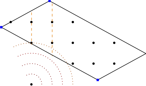
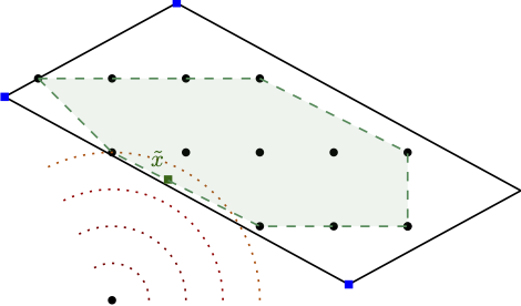
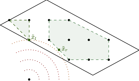
Figure 1. Solving stronger subproblems, directly optimizing over the mixed-integer hull can be very powerful. (left) baseline and fractional optimal solution, (middle-left) branching on fractional variable leads only to minor improvement, (middle-right) direct optimization over the mixed-integer hull and fractional solution over the mixed-integer hull, (right) branching once results in optimal solution.
As such, our approach is a Mixed-Integer Conditional Gradient Algorithm that combines a specific Frank-Wolfe algorithm, the Blended Pairwise Conditional Gradient (BPCG) approach of [TTP] (see also the earlier BPCG post), with a branch-and-bound scheme, and solves MIPs as LMOs. Our approach combines several very powerful improvements from conditional gradients with state-of-the-art MIP techniques to obtain a fast algorithm.
Tricks to make it work
- Leveraging MIP improvements. As our LMOs in the FW subsolver are standards MIPs we can exploit the whole toolbox of MIP solver improvements. In particular, we can use solution pools to collect and reuse previously identified feasible solution. Note, that as our feasible region is never modified (in contrast to, e.g., outer approximation relying on epigraph formulations), all discovered primal solution are globally feasible. In future releases we will also support more advanced reoptimization features of modern MIP solvers, such as carrying over certain presolve information, propagation, and cutting planes.
- Incomplete resolution of nodes. We do not have to solve nodes to near-optimality but rather we can use an adaptive gap strategy to only partially resolve subproblems, significantly reducing the number of iterations in the FW subsolver.
- Warmstarting. We can warmstart the FW subsolver from the run before branching, further cutting down required iterations. For this we can efficiently (as in: for free) write the parent solution as a convex combination of two distinct solutions valid for the left and the right branch, respectively.
- Lazification and blending. We generalize both the lazification [BPZ] and blending approach [BPTW] to apply to the whole tree allowing to aggressively reuse previously found primal feasible solutions. In particular, no primal feasible solution has to be computed or discovered twice.
- Hybrid branching strategy. Finally, we developed a hybrid branching strategy that can further reduce the number of required nodes; however this is highly dependend on the instance.
Combining and exploiting all these things, this results in having only to solve something like 5-8 LMOs calls per node on average and the longer the run and the deeper the tree, the smaller this number is. Asymptotically the average number of LMO calls is approaching something close to 1 as no MIP-feasible solution is computed twice as mentioned above. For a more complex instance, the overall impact of these tricks is shown in Figure 2 below in terms of the average number of LMO calls per node.
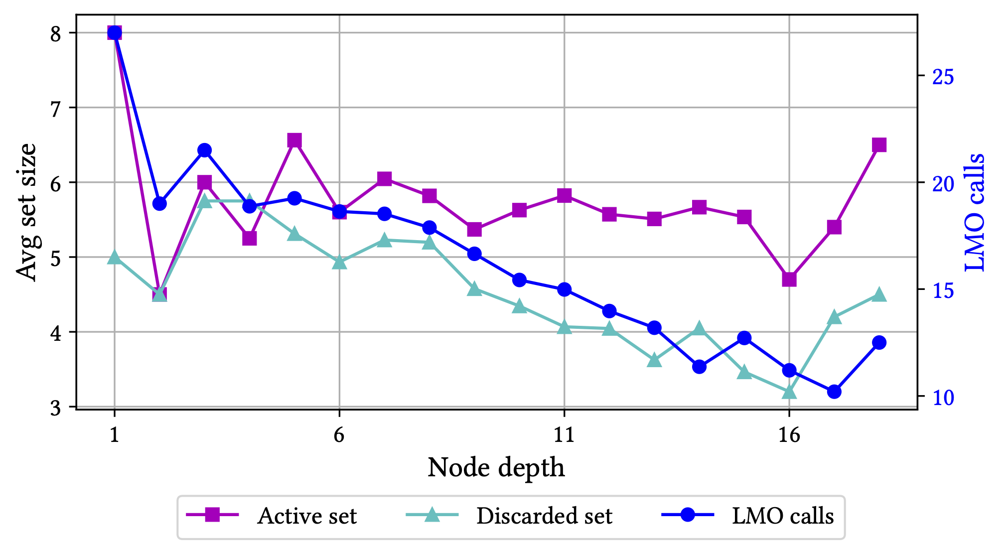
Figure 2. Minimizing a quadratic over a cardinality constrained variant of the Birkhoff polytope. Key statistics as a function of the node depth. Both the size of the active (vertex) set and the discarded (vertex) set remain small throughout the run of the algorithm and the average number of LMO calls required to solve a subproblem drops significantly as a function of depth as previously discovered solutions cut out unnecessary LMO calls.
For more details see the preprint [HTBP].
Implementation of Boscia.jl in a nutshell
- Released under MIT license. Do whatever you want with it and consider contributing to the code base.
- Uses our earlier
FrankWolfe.jlJulia package as well theBonobo.jlbranch-and-bound Julia package. - Uses the Blended Pairwise Conditional Gradient (BPCG) algorithm [TTP] together with (a modified variant of) the adaptive step-size strategy of [PNAJ] from the
FrankWolfe.jlpackage. - Supports a wide variety of MIP solvers through the MathOptInterface (MOI). Currently, we use
SCIP.jlwith SCIP 8 in our examples. - via MOI reads .mps and .lp files out of the box allowing to easily replace linear objectives by convex objectives.
- Interface is identical to that of
FrankWolfe.jl: specify the objective and its gradients and provide an LMO for the feasible region.
Contribute
Most certainly there will be still bugs, calibration issues, and numerical issues in the solver. Any feedback, bug reports, issues, PRs are highly welcome on the package’s github repository.
A simple example
using Boscia
using FrankWolfe
using Random
using SCIP
using LinearAlgebra
import MathOptInterface
const MOI = MathOptInterface

n = 6

const diffw = 0.5 * ones(n)

##############################
# defining the LMO and using
# SCIP as solver for the LMO
##############################

o = SCIP.Optimizer()

MOI.set(o, MOI.Silent(), true)

x = MOI.add_variables(o, n)

for xi in x
    MOI.add_constraint(o, xi, MOI.GreaterThan(0.0))
    MOI.add_constraint(o, xi, MOI.LessThan(1.0))
    MOI.add_constraint(o, xi, MOI.ZeroOne())
end

lmo = FrankWolfe.MathOptLMO(o) # MOI-based LMO

##############################
# defining objective and
# gradient
##############################

function f(x)
    return sum(0.5*(x.-diffw).^2)
end

function grad!(storage, x)
    @. storage = x-diffw
end


##############################
# calling the solver
##############################

x, _, result = Boscia.solve(f, grad!, lmo, verbose = true)
The output - which is quite wide - then roughly looks like this:
Boscia Algorithm.

Parameter settings.
	 Tree traversal strategy: Move best bound
	 Branching strategy: Most infeasible
	 Absolute dual gap tolerance: 1.000000e-06
	 Relative dual gap tolerance: 1.000000e-02
	 Frank-Wolfe subproblem tolerance: 1.000000e-05
	 Total number of varibales: 6
	 Number of integer variables: 0
	 Number of binary variables: 6


---------------------------------------------------------------------------------------------------------------------------------------------------------------------------------------------------
   Iteration       Open          Bound      Incumbent      Gap (abs)      Gap (rel)       Time (s)      Nodes/sec        FW (ms)       LMO (ms)  LMO (calls c)   FW (Its)   #ActiveSet  Discarded
---------------------------------------------------------------------------------------------------------------------------------------------------------------------------------------------------
*          1          2  -1.202020e-06   7.500000e-01   7.500012e-01            Inf   3.870000e-01   7.751938e+00            237              2              9         13            1          0
         100         27   6.249998e-01   7.500000e-01   1.250002e-01   2.000004e-01   5.590000e-01   2.271914e+02              0              0            641          0            1          0
         127          0   7.500000e-01   7.500000e-01   0.000000e+00   0.000000e+00   5.770000e-01   2.201040e+02              0              0            695          0            1          0
---------------------------------------------------------------------------------------------------------------------------------------------------------------------------------------------------

Postprocessing

Blended Pairwise Conditional Gradient Algorithm.
MEMORY_MODE: FrankWolfe.InplaceEmphasis() STEPSIZE: Adaptive EPSILON: 1.0e-7 MAXITERATION: 10000 TYPE: Float64
GRADIENTTYPE: Nothing LAZY: true lazy_tolerance: 2.0
[ Info: In memory_mode memory iterates are written back into x0!

----------------------------------------------------------------------------------------------------------------
  Type     Iteration         Primal           Dual       Dual Gap           Time         It/sec     #ActiveSet
----------------------------------------------------------------------------------------------------------------
  Last             0   7.500000e-01   7.500000e-01   0.000000e+00   1.086583e-03   0.000000e+00              1
----------------------------------------------------------------------------------------------------------------
    PP             0   7.500000e-01   7.500000e-01   0.000000e+00   1.927792e-03   0.000000e+00              1
----------------------------------------------------------------------------------------------------------------

Solution Statistics.
	 Solution Status: Optimal (tree empty)
	 Primal Objective: 0.75
	 Dual Bound: 0.75
	 Dual Gap (relative): 0.0

Search Statistics.
	 Total number of nodes processed: 127
	 Total number of lmo calls: 699
	 Total time (s): 0.58
	 LMO calls / sec: 1205.1724137931035
	 Nodes / sec: 218.96551724137933
	 LMO calls / node: 5.503937007874016
References
[TTP] Tsuji, K., Tanaka, K. I., & Pokutta, S. (2021). Sparser kernel herding with pairwise conditional gradients without swap steps. to appear in Proceedings of ICML. arXiv preprint arXiv:2110.12650. pdf
[PNAJ] Pedregosa, F., Negiar, G., Askari, A., & Jaggi, M. (2020, June). Linearly convergent Frank-Wolfe with backtracking line-search. In International Conference on Artificial Intelligence and Statistics (pp. 1-10). PMLR. pdf
[BDRT] Buchheim, C., De Santis, M., Rinaldi, F., & Trieu, L. (2018). A Frank–Wolfe based branch-and-bound algorithm for mean-risk optimization. Journal of Global Optimization, 70(3), 625-644. pdf
[HTBP] Hendrych, D., Troppens, H., Besançon, M., & Pokutta, S. (2022). Convex integer optimization with Frank-Wolfe methods. arXiv preprint arXiv:2208.11010. pdf
[BPTW] Braun, G., Pokutta, S., Tu, D., & Wright, S. (2019, May). Blended conditonal gradients. In International Conference on Machine Learning (pp. 735-743). PMLR. pdf
[BPZ] Braun, G., Pokutta, S., & Zink, D. (2017, July). Lazifying conditional gradient algorithms. In International conference on machine learning (pp. 566-575). PMLR. pdf
Comments