Non-Convex Boosting via Integer Programming
TL;DR: This is an informal summary of our recent paper IPBoost – Non-Convex Boosting via Integer Programming with Marc Pfetsch, where we present a non-convex boosting procedure that relies on integer programing. Rather than solving a convex proxy problem, we solve the actual classification problem with discrete decisions. The resulting procedure achieves performance at par or better than Adaboost however it is robust to label noise that can defeat convex potential boosting procedures.
What is the paper about and why you might care
Boosting (see Wikipedia) is an important (and by now standard) technique in classification to combine several “low accuracy” learners, so-called base learners, into a “high accuracy” learner, a so-called boosted learner. Pioneered by the AdaBoost approach of [FS], in recent decades there has been extensive work on boosting procedures and analyses of their limitations. In a nutshell, boosting procedures are (typically) iterative schemes that roughly work as follows: for $t = 1, \dots, T$ do the following:
- Train a learner $\mu_t$ from a given class of base learners on the data distribution $\mathcal D_t$.
- Evaluate performance of $\mu_t$ by computing its loss.
- Push weight of the data distribution $\mathcal D_t$ towards misclassified examples leading to $\mathcal D_{t+1}$.
Finally, the learners are combined by some form of voting (e.g., soft or hard voting, averaging, thresholding). A close inspection of most (but not all) boosting procedures reveals that they solve an underlying convex optimization problem over a convex loss function by means of coordinate gradient descent. Boosting schemes of this type are often referred to as convex potential boosters. These procedures can achieve exceptional performance on many data sets if the data is correctly labeled. In fact, in theory, provided the class of base learners is rich enough, a perfect strong learner can be constructed that has accuracy $1$ (see e.g., [AHK]), however clearly such a learner might not necessarily generalize well. Boosted learners can generate quite some complicated decision boundaries, much more complicated than that of the base learners. Here is an example from Paul van der Laken’s blog / Extreme gradient boosting gif by Ryan Holbrook. Here data is generated online according to some process with optimal decision boundary represented by the dotted line and XGBoost was used learn a classifier:

Label noise
In reality we usually face unclean data and so-called label noise, where some percentage of the classification labels might be corrupted. We would also like to construct strong learners for such data. However if we revisit the general boosting template from above, then we might suspect that we run into trouble as soon as a certain fraction of training examples is misclassified: in this case these examples cannot be correctly classified and the procedure shifts more and more weight towards these bad examples. This eventually leads to a strong learner, that perfectly predicts the (flawed) training data, however that does not generalize well anymore. This intuition has been formalized by [LS] who construct a “hard” training data distribution, where a small percentage of labels is randomly flipped. This label noise then leads to a significant reduction in performance of these boosted learners; see tables below. The more technical reason for this problem is actually the convexity of the loss function that is minimized by the boosting procedure. Clearly, one can use all types of “tricks” such as early stopping but at the end of the day this is not solving the fundamental problem.
Our results
To combat the problem of convex potential boosters being susceptible to label noise, rather than optimizing some convex loss proxy, why not considering the classification problem with the actual misclassification loss function:
\[\tag{classify} \begin{align} \label{eq:trueLoss} \ell(\theta,D) \doteq \sum_{i \in I} \mathbb I[h_\theta(x_i) \neq y_i], \end{align}\]where $h_\theta$ is a learner parameterized by $\theta$ and $D = \setb{(x_i,y_i) \mid i \in I}$ is the training data? This loss function counts the number of misclassifications, which somehow seems to be a natural quantity to minimize. Unfortunately, this loss function is non-convex, however, the resulting optimization problem can be rather naturally phrased as an Integer Program (IP). In fact, our basic boosting model is captured by the following integer programming problem:
\[\tag{basicBoost} \begin{align*} \min\; & \sum_{i=1}^N z_i \\ & \sum_{j=1}^L \eta_{ij}\, \lambda_j + (1 + \rho) z_i \geq \rho\quad\forall\, i \in [N],\\ & \sum_{j=1}^L \lambda_j = 1,\; \lambda \geq 0,\\ & z \in \{0,1\}^N, \end{align*}\]where the matrix $\eta_{ij}$ encodes the predictions of learner $j$ on example $i$. The boosting part comes naturally into play here as the number of base learners is potentially huge (sometimes even infinite) and we have to generate these learners with some procedure. We do this by means of column generation, where we add base learners via a pricing problem, that essentially generates an acceptable base learner for the modified data distribution that is encoded in the dual variables of the relaxed problem (basicBoost). This is somewhat similar to the (LP-based) LPBoost approach of [DKS] however we consider an integer program here where column generation is significantly more involved. The dual problem is of the following form:
\[\begin{align*} \tag{dualProblem} \max\; & \rho \sum_{i=1}^N w_i + v - \sum_{i=1}^N u_i\\ & \sum_{i=1}^N \eta_{ij}\, w_i + v \leq 0 \quad\forall\, j \in \mathcal{L},\\ & \;(1 + \rho) w_i - u_i \leq 1\quad\forall\, i \in [N],\\ & w \geq 0,\; u \geq 0,\; v \text{ free}, \end{align*}\]and after some clean up etc, the pricing constraints that need to be satisfied are:
\[\tag{pricing} \begin{equation}\label{eq:PricingProb} \sum_{i=1}^N \eta_{ij}\, w_i^\esx + v^\esx > 0 \end{equation},\]and we ask whether there exist a base learner $h_j \in \Omega$ such that (pricing) holds? For this, the $w_i^\esx$ can be seen as weights over the points $x_i$ with $i \in [N]$, and we have to classify the points according to these weights. This pricing problem is solved within a branch-and-cut-and-price framework, complicating things significantly compared to column generation in the LP case.
Computations
Solving an IP is much more computationally expensive than traditional boosting approaches or LPBoost. However, what we gain is robustness and stability. For the hard distribution of [LS] we significantly outperform Adaboost and gain moderately compared to LPBoost, which is already more robust towards label noise as it re-solves the optimization in each round, albeit for a proxy loss function. The reported accuracy is test accuracy over multiple runs for various parameters and $L$ denotes the (average) number of learners generated in order to construct the strong learner.
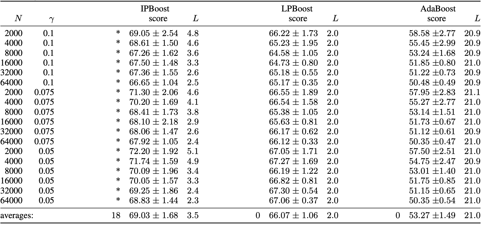
Note that the hard distribution is for a binary classification problem, so that $50\%$ accuracy is random guessing. Therefore the improvement from $53.27\%$ for Adaboost, which is basically random guessing to $69.03\%$ is quite significant.
References
[FS] Freund, Y., & Schapire, R. E. (1995, March). A desicion-theoretic generalization of on-line learning and an application to boosting. In European conference on computational learning theory (pp. 23-37). Springer, Berlin, Heidelberg. pdf
[AHK] Arora, S., Hazan, E., & Kale, S. (2012). The multiplicative weights update method: a meta-algorithm and applications. Theory of Computing, 8(1), 121-164. pdf
[LS] Long, P. M., & Servedio, R. A. (2010). Random classification noise defeats all convex potential boosters. Machine learning, 78(3), 287-304. pdf
[DKS] Demiriz, A., Bennett, K. P., & Shawe-Taylor, J. (2002). Linear programming boosting via column generation. Machine Learning, 46(1-3), 225-254. pdf
Comments