Conditional Gradients and Acceleration
TL;DR: This is an informal summary of our recent paper Locally Accelerated Conditional Gradients [CDP] with Alejandro Carderera and Jelena Diakonikolas, showing that although optimal global convergence rates cannot be achieved for Conditional Gradients [CG], acceleration can be achieved after a burn-in phase independent of the accuracy $\epsilon$, giving rise to asymptotically optimal rates, accessing the feasible region only through a linear minimization oracle.
Written by Alejandro Carderera.
In this post we will consider optimization problems of the form
\[\min_{x \in P} f(x),\]where $f$ is an $L$-smooth convex or $\mu$-strongly convex function and $P$ is a polytope (in particular compact and convex). We will denote a solution to this problem as $x^\esx = \arg\min_{x \in P} f(x)$; note that the solution is unique in the $\mu$-strongly convex case.
In the previous blog post Cheat Sheet: Acceleration from First Principles we saw that we can achieve acceleration (going from $\mathcal{O} ( \frac{L}{\mu} \log \frac{1}{\epsilon} )$ to $\mathcal{O} ( \sqrt{\frac{L}{\mu}} \log \frac{1}{\epsilon} )$ iterations for $L$-smooth $\mu$-strongly convex functions and from $\mathcal{O} (1/\epsilon )$ to $\mathcal{O} ( 1/\sqrt{\epsilon} )$ iterations for (general) $L$-smooth convex functions to achieve an accuracy of $\epsilon$) by simultaneously optimizing the primal and dual update, as opposed to only optimizing the primal or dual update, as vanilla gradient descent and mirror descent do, respectively. A natural question to ask is, can Conditional Gradients (CG) [CG, FW] be accelerated in that same spirit? This would effectively mean that we have a projection-free first-order constrained optimization algorithm with optimal convergence rates for smooth convex and strongly convex functions. Let’s explore the matter in more depth; we only consider the strongly convex case in the following.
Global Acceleration: A fundamental barrier
Can we achieve accelerated convergence rates globally for CG, i.e., can they hold for all problem instances, throughout the whole algorithm? Let us start with the example already considered in previous posts (Cheat Sheet: Frank-Wolfe and Conditional Gradients and Cheat Sheet: Linear convergence for Conditional Gradients) which was studied in depth in terms of complexity in [L].
Example: Consider the function $f(x) \doteq \norm{x}^2$, which is strongly convex and the polytope $P = \mathrm{conv} \setb{ e_1,\dots, e_n} \subseteq \mathbb{R}^n$, the probability simplex in dimension $n$. We want to solve $\min_{x \in P} f(x)$. Clearly, the optimal solution is $x^\esx = (\frac{1}{n}, \dots, \frac{1}{n})$. Recall that at each iteration we call the first-order oracle to obtain a gradient, and the linear optimization oracle to solve a linear program. Whenever we call the linear programming oracle, we will obtain one of the $e_i$ vectors and in lieu of any other information but that the feasible region is convex, we can only form convex combinations of those. Thus after $t$ iterations, the best we can produce as a convex combination is a vector with support $t$, where the minimizer of such vectors for $f(x)$ is, e.g., $x_t = (\frac{1}{t}, \dots,\frac{1}{t},0,\dots,0)$ with $t$ times $1/t$ entries, so that we obtain a gap \(h(x_t) \doteq f(x_t) - f(x^\esx) \geq \frac{1}{t}-\frac{1}{n},\) which after requiring $\frac{1}{t}-\frac{1}{n} < \varepsilon$ implies $t > \frac{1}{\varepsilon - 1/n} \approx \frac{1}{\varepsilon}$ for $n$ large. In particular for $t = n/2$, assuming even $n$ it holds that: \[h(x_{t}) \geq \frac{1}{t}-\frac{1}{n} = \frac{1}{2t}.\]
As is clear from this lower bound on the primal gap, a convergence rate of $O(1/\sqrt{t})$ cannot be attained in general. Moreover, note that the objective function is strongly convex. Recall from post Cheat Sheet: Linear convergence for Conditional Gradients that an algorithm has a linear convergence rate if it contracts the primal gap as $f(x_t) - f^\esx \leq e^{-rt} (f(x_0) - f^\esx)$ with $r>0$. If we apply the previous lower bound to a convergence rate of this form for $t = n/2$, i.e., $1/2t \leq f(x_t) - f^\esx \leq e^{-rt} (f(x_0) - f^\esx)$, and we note that $f(x_0) - f^\esx \leq 1$, we arrive at $r \leq 2 \frac{\log 2t}{2t}$. Consider the linearly convergent primal gap evolution of the Fully-Corrective Frank-Wolfe variant [LJ], which has the form $f(x_t) - f^\esx \leq \left(1 - \frac{\mu}{4L} \left( \frac{w(P)}{D} \right)^2 \right)^t (f(x_0) - f^\esx)$, where $w(P)$ is the pyramidal width of $P$ and $D$ is the diameter of $P$. For the problem instance we are considering with $D = \sqrt{2}$, $\mu = L = 1$, and $w(P) = 2/\sqrt{n}$ we arrive at the fact that $r = \frac{1}{2n} = \frac{1}{4t}$. Therefore we see that at most the convergence rate of this Frank-Wolfe variant can only be improved up to a logarithmic factor, and a convergence rate of $\mathcal{O} ( \sqrt{\frac{L}{\mu}} \log \frac{1}{\epsilon} )$ is not globally attainable in terms of calls to the linear optimization oracle. Similar conclusions can be drawn for the Away-Step and Pairwise-Step Frank Wolfe algorithms.
Despite the previous global conclusion in terms of linear optimization oracle calls, the Conditional Gradient Sliding algorithm [LZ] achieves an optimal convergence rate in terms of global first-order oracle calls, requiring $\mathcal{O} ( \sqrt{\frac{L}{\mu}} \log \frac{1}{\epsilon} )$ first-order oracle calls, i.e., gradient evaluations, and $\mathcal{O} ( \frac{L}{\mu} \log \frac{1}{\epsilon} )$ linear optimization oracle calls to achieve an accuracy of $\epsilon$ for $L$-smooth and $\mu$-strongly convex functions. In light of the barrier to global acceleration, can we achieve acceleration in terms of calls to the linear optimization oracle locally with CG? Bear in mind that the lower bound holds only up to the dimension $n$. As such, this bound does not answer the question of whether true acceleration is possible beyond the dimension with respect to both first-order oracle calls and linear optimization oracle.
Local Acceleration beyond the Dimension
As the title of this post already suggests, an optimal convergence rate can be achieved with CG, but only locally. We will call this algorithm the Locally Accelerated Conditional Gradient algorithm, obtained as the combination of a linearly convergent CG method and a novel accelerated algorithm. The key ingredient is a Generalized Accelerated Method, an extension of the $\mu AGD+$ algorithm from [CDO], which we call the Modified $\mu AGD+$ algorithm, that can be coupled with an alternative algorithm (in this case CG, which is run independently), in such a way that at each iteration the point with lowest objective function value is chosen. The Modified $\mu AGD+$ is run on the convex hull of a set $\mathcal{C}$ (and therefore the point from the alternative algorithm also has to be in $\mathcal{C}$), and if $x^\esx \in \operatorname{conv} \mathcal{C}$ it will converge to $x^\esx$ with an optimal convergence rate in terms of first-order oracle and linear optimization oracle calls. However we cannot include all the vertices of $P$ in $\mathcal{C}$ as then each step of the Modified $\mu AGD+$ algorithm will be prohibitively expensive; note that a polytope can have a number of vertices exponential in the dimension. Ideally what we want is for $\mathcal{C}$ to be formed by the minimum number of vertices of $P$, such that $x^\esx \in \operatorname{conv} \mathcal{C}$ and we know the cardinality of this set should be at most $n+1$ by Carathéodory’s theorem. Note that the use of the Modified $\mu AGD+$ algorithm relaxes the projection-free requirement of the algorithm, as at each iteration it has to solve a convex subproblem over the convex hull of the elements in $\mathcal{C}$ (which will be equivalent to solving a projection problem over a simplex of low dimension).
Let us denote by $\mathcal{C}_t$ the set $\mathcal{C}$ at iteration $t$. The high-level description from above brings to mind the following question: How do we select $\mathcal{C}_t$ at each iteration $t$? This is where the CG algorithm comes in. Consider choosing a CG variant such as the Away-Step Frank-Wolfe (AFW) algorithm with the short-step rule (as detailed in Cheat Sheet: Frank-Wolfe and Conditional Gradients). The AFW algorithm maintains its iterates $x_t^{\text{AFW}}$ as a convex combination of the extreme points of $P$. Let us denote by $\mathcal{S}_t^{\text{AFW}}$ the set of these vertices,
\[\mathcal{S}_t^{\text{AFW}} = \setb{ \setb{v_1, \cdots, v_m} \;\vert\; v_i \in P, \lambda_{i} > 0 \; \forall i \in [1,\cdots ,m]; x_t^{\text{AFW}} = \sum_{j = 1}^{m} \lambda_{j}v_j, \sum_{j = 1}^{m} \lambda_{j} =1}.\]We also know that by the finiteness of the number of active sets and the closedness of P there exists $r>0$ and $T \in \mathbb{N}_+$ such that $\norm{x_t^{\text{AFW}} - x^\esx} < r$ and $x^\esx \in \mathcal{S}_t^{\text{AFW}}$ for all $t \geq T$. The values of $r$ and $T$ are independent of $\epsilon$ and depend only on $f$ and $P$. It therefore seems natural to consider the $\mathcal{S}_t^{\text{AFW}}$ as potential candidates for $\mathcal{C}_t$, i.e., the CG algorithm is used to identify a small active set such that $x^\esx \in \operatorname{conv} \mathcal{C}$, in what we will call a burn-in phase, after which the Modified $\mu AGD+$ algorithm will drive the iterates with optimal convergence rate.
However, we do not know a priori what the value of $T$ is, and we have no way of certifying that for a given iteration $t$ we have $x^\esx \in \operatorname{conv}\mathcal{S}_t^{\text{AFW}}$. Otherwise we could just simply run AFW for $T$ iterations, set \(\mathcal{C}_t = \mathcal{S}_T^{\text{AFW}},\) and then run the Modified $\mu AGD+$ algorithm in the convex hull of \(\mathcal{C}_t\) from then onwards. This is why LaCG runs the AFW algorithm and the Modified $\mu AGD+$ algorithm simultaneously, updating the set \(\mathcal{C}_{t}\) relative to \(\mathcal{S}_t^{\text{AFW}}\) or restarting the Modified $\mu AGD+$ algorithm when certain conditions are met. As long as $t \leq T$ the convergence is driven by AFW, and once $t >T$ the convergence is driven by the Modified $\mu AGD+$ algorithm. Note that we still restart the accelerated sequence even when $t > T$ (simply because we do not know when we have reached T), however the restarts are delayed to ensure sufficient progress is made (losing at most a factor of 2 in the convergence rate); in practice this regime shift might actually happen already before reaching $T$.
As the careful reader will have noticed, at each iteration we’ll be performing an AFW step, and a Modified $\mu AGD+$ step. And when $x^\esx \in \operatorname{conv} \mathcal{C}_{t}$, LaCG will have a convergence rate of $\mathcal{O} ( \sqrt{\frac{L}{\mu}} \log \frac{1}{\epsilon} )$ for L-smooth and $\mu$-strongly convex functions, as opposed to $\mathcal{O} ( \frac{L}{\mu} \log \frac{1}{\epsilon} )$ for AFW, so we’ll have greater progress-per-iteration compared to AFW. Note also that the accelerated convergence rate we obtain is independent of the dimension $n$. This is not the case for the Catalyst-augmented variant we benchmark against as we will see below. But how will we perform in terms of wall-clock time?
Computational Experiments
We consider three different feasible regions $P$:
- Probability Simplex $\Delta$
- $\ell_1$-unit ball.
- Birkhoff polytope.
Note that for all instances shown considered here the global minimum of the objective function will not be contained in the feasible region $P$, and therefore the constrained optimum will lie on the boundary of $P$.
Optimization over the probability simplex
Let’s see how our algorigthm performs in practice. Consider an $L$-smooth and $\mu$-strongly quadratic of the form $f(x) = x^T Mx$, with $L / \mu = 1000$ and $x \in \mathbb{R}^n$ for $n=2000$. Our feasible region $P$ will be the probability simplex (note that this case could also be easily handled with projected AGD). The following image shows on top the normalized primal gap $h(x_t)/h(x_0)$ in terms of the number of iterations for three different methods: the LaCG algorithm, the AFW algorithm, and a Catalyst-augmented AFW algorithm [LMH], which has a global convergence rate in terms of linear oracle calls of $\mathcal{O} ( \sqrt{\frac{L}{\mu}} \frac{D^2}{\delta^2} \log \frac{1}{\epsilon} )$. The image on the bottom shows the percentage of optimal vertices (those that are required to write the optimal solution as a convex combination) that have been picked up by the AFW algorithm, when the black line reaches $100\%$ on the y-axis, it means that \(x^\esx \in \operatorname{conv} S_{t}^{\text{AFW}},\) and therefore if we would pick \(\mathcal{C}_{t} = S_{t}^{\text{AFW}}\) we’ll observe our sought-after acceleration, i.e., a sharp speed-up in convergence. Observe that the LaCG algorithm does not require knowledge of the optimal active set, and there could be multiple optimal and minimal active sets. The black dots indicate the iterations at which the LaCG restarts the Modified $\mu AGD+$ algorithm, and we set \(\mathcal{C}_{t} = S_{t}^{\text{AFW}}\).
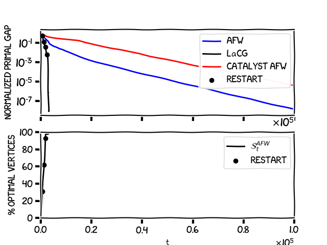
As mentioned previously, the LaCG algorithm makes at least as much progress per iteration as AFW. However, we can see in the graph that the algorithm makes substantially more progress per iteration than AFW, even before it has had time to pick up all the optimal vertices; we have partial acceleration already on the sub-optimal active sets. We can also observe that the Catalyst-augmented AFW has a pretty slow convergence rate, looking carefully at the fact that $D^2 = 2$ and $\delta^2 = 4/n$ for the simplex we arrive at $\frac{D^2}{\delta^2} = 1000$, leading to the observation that $\sqrt{\frac{L}{\mu}} \frac{D^2}{\delta^2} \geq \frac{L}{\mu}$ in the convergence rate for this problem instance. This inevitable dimension dependence is one of the shortcomings of the Catalyst method, and it is also the reason why this method does not violate the lower bound we mentioned previously and can obtain global convergence rates that depend on $\sqrt{\frac{L}{\mu}}$. The following image shows the behavior of the algorithms in terms of wall-clock time.
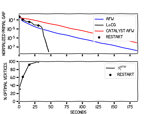
The beauty of LaCG is that due to the small dimensionality of the sets \(\mathcal{C}_{t}\), we can perform the Modified $\mu AGD+$ steps efficiently, and even when we have not picked up all the optimal vertices, we are still competitive with AFW in terms of wall-clock time. Note the speed-up seen in the previous plot once \(x^\esx \in \mathcal{C}_{t}\).
Optimization over the $\ell_1$-unit ball
The $\ell_1$ ball is often encountered in Lasso regression problems, where the aim is to find an accurate yet interpretable solution to a least-squares problem. In this example the feasible region will be the $\ell_1$-unit ball, and the objective function will again be a quadratic of the same form with a global minimum outside of the $\ell_1$-unit ball, with $L / \mu = 100$ and $x \in \mathbb{R}^n$ for $n=2000$. The following experiments were run for $240$ seconds of wall-clock time.
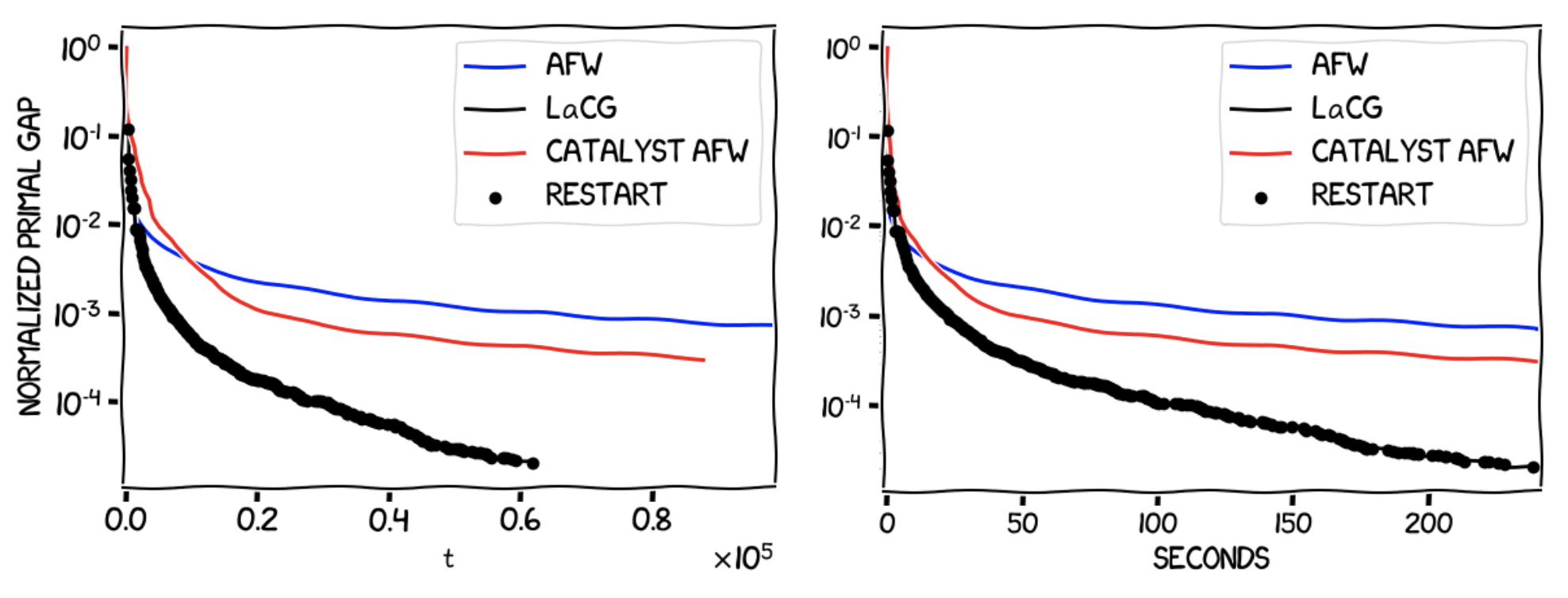
As was the case for the probability simplex, LaCG outperforms both AFW and the Catalyst-augmented AFW algorithm in terms of progress per iteration and wall-clock time, outputting a solution that is more than an order of magnitude higher in accuracy in the same wall-clock time interval.
Optimization over the Birkhoff polytope
The Birkhoff polytope, also called the polytope of doubly stochastic matrices, or assignment polytope, is formed by the square matrices $Q \in \mathbb{R}^{n \times n}$ such that each row/column in the matrix sums up to $1$. Its vertices are the $n!$ permutation matrices, which are matrices in $\mathbb{R}^{n \times n}$ that have exactly one entry equal to $1$ in each row and in each column, being the entries elsewhere equal to $0$. Projection in the Euclidean sense onto this polytope is not as easy as projecting onto the probability simplex, which makes projection-free methods like CG and LaCG of considerable interest. Consider again an $L$-smooth and $\mu$-strongly quadratic of the form $f(x) = x^T Mx$, with $L / \mu = 100$ and $x \in \mathbb{R}^{n \times n}$ for $n \times n = 1600$. Now our feasible region $P$ will be the Bikhoff polytope. The following images show the evolution of the normalized primal gap $h(x_t)/h(x_0)$ in terms of iterations and in terms of wall-clock time.
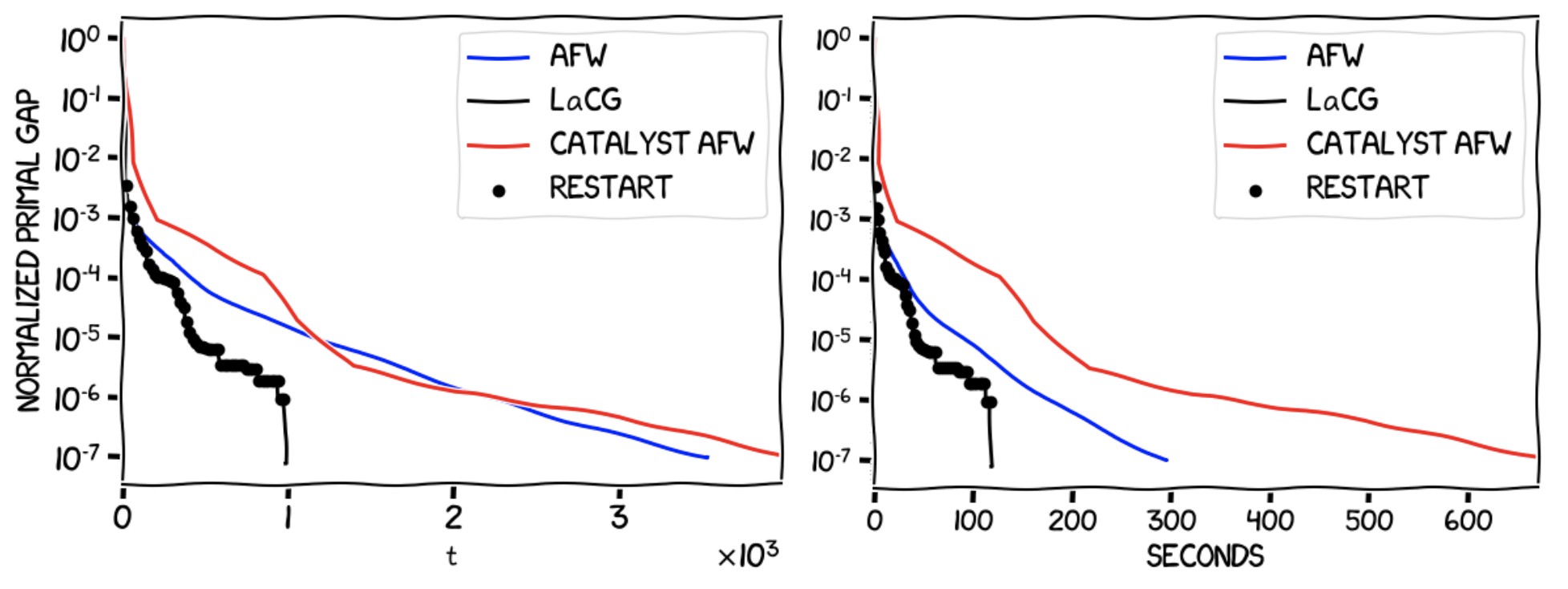
As we saw in the example with the simplex, LaCG outperforms both AFW and the Catalyst-augmented AFW algorithm in terms of progress per iteration, and in terms of wall-clock time, even before the optimal face has been identified (which happens at approximately $t = 1000$). After this has happened, we see a phenomenal performance boost in both metrics. As before, note the effect of the dimension dependence of the convergence rate of the Catalyst-augmented AFW algorithm. This can be further seen in the following image, which shows a quadratic with the same $L/\mu$ over the Birkhoff polytope in $\mathbb{R}^{n \times n}$ for a smaller dimension $n \times n = 400$.
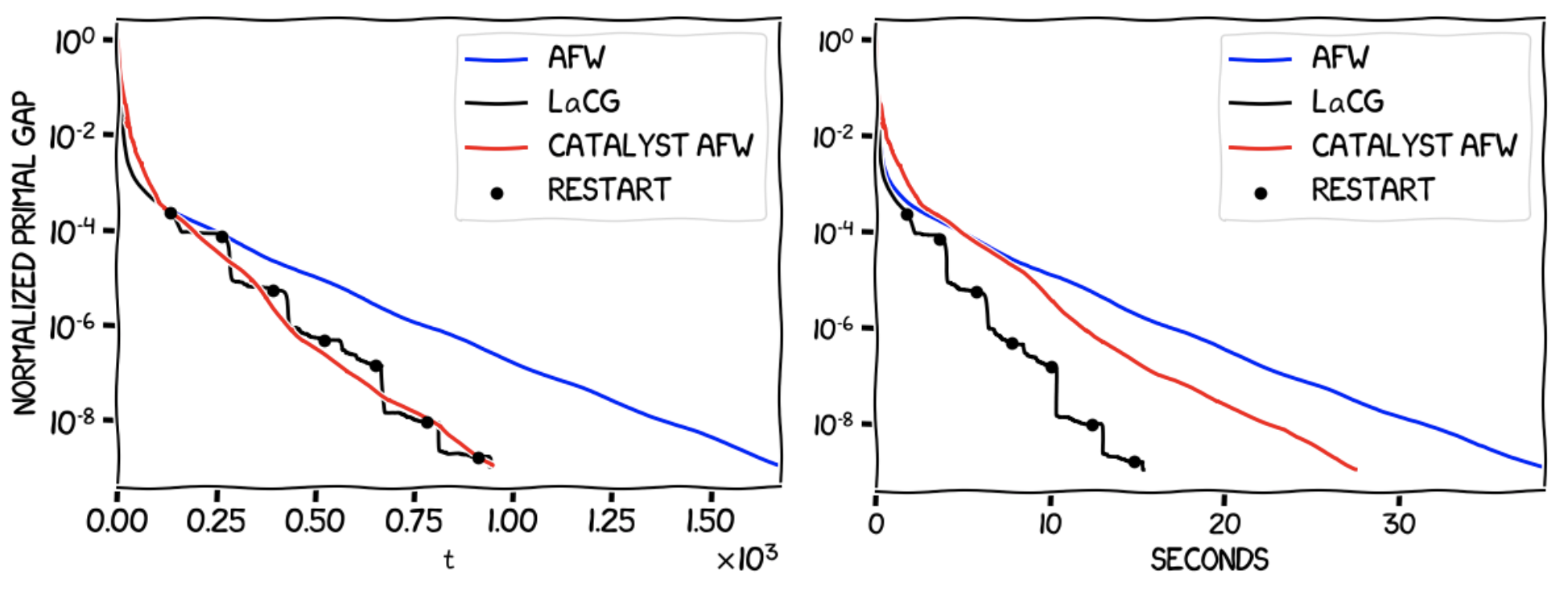
For lower dimensions, the Catalyst-augmented AFW becomes competitive with LaCG in terms of progress per iteration, however LaCG performs much better in terms of wall-clock time. Another thing to note is the stair-like behaviour of the LaCG algorithm. This is due to the fact that between the restarts (the black circles in the image), we do not change the elements in \(\mathcal{C}_{t}\), and LaCG converges to a solution of \(\min_{x \in \mathcal{C}_{t}} f(x)\), and we cannot guarantee that \(x^\esx \in \operatorname{conv} \mathcal{C}_{t}\), however due to the delayed restarts LaCG resets $\mathcal{C}_{t}$ often enough and converges to $x^\esx$ faster than AFW and the Catalyst-augmented AFW algorithm.
Some other important features of LaCG are:
- The Modified $\mu AGD+$ subproblems at each time step do not have to be solved to perfect optimality, instead they can be solved approximately to a tolerance $\epsilon_t$ (more details can be found in [CDP]).
- If we use a projection-free algorithm to solve the subproblems in the Modified $\mu AGD+$ step, we arrive at a fully projection-free algorithm. We recover a variant of the Conditional Gradient Sliding [LZ] algorithm: ignore the AFW steps in the LaCG algorithm, only perform Modified $\mu AGD+$ steps, and solve the subproblems with a CG algorithm.
References
[CDP] Carderera, A., Diakonikolas, J., Pokutta, S., (2019). Locally Accelerated Conditional Gradients. arXiv preprint arXiv:1906.07867. pdf
[CG] Levitin, E. S., & Polyak, B. T. (1966). Constrained minimization methods. Zhurnal Vychislitel’noi Matematiki i Matematicheskoi Fiziki, 6(5), 787-823. pdf
[FW] Frank, M., & Wolfe, P. (1956). An algorithm for quadratic programming. Naval research logistics quarterly, 3(1‐2), 95-110. pdf
[L] Lan, G., (2013). The complexity of large-scale convex programming under a linear optimization oracle. arXiv preprint arXiv:1309.5550. pdf
[LJ] Lacoste-Julien, S., & Jaggi, M. (2015). On the global linear convergence of Frank-Wolfe optimization variants. In Advances in Neural Information Processing Systems (pp. 496-504). pdf
[LZ] Lan, G. and Zhou, Y., (2016). Conditional gradient sliding for convex optimization. SIAM Journal on Optimization, 26(2), pp.1379-1409. pdf
[CDO] M. B. Cohen, J. Diakonikolas, and L. Orecchia, (2018). On acceleration with noise-corrupted gradients. In Proc. ICML’18. pdf
[LMH] Lin, H., Mairal, J. and Harchaoui, Z., (2015). A universal catalyst for first-order optimization. In Advances in Neural Information Processing Systems (pp. 3384-3392). pdf
Comments