Cheat Sheet: Acceleration from First Principles

TL;DR: Cheat Sheet for a derivation of acceleration from optimization first principles.

Posts in this series (so far).

My apologies for incomplete references—this should merely serve as an overview.

Acceleration in smooth convex optimization has been met with awe and has been subject to extensive research over the last years. In a nutshell, what acceleration does is that it provides an “unexpected” speedup in smooth convex optimization; we will be concerned with acceleration in the Nesterov sense [N1], [N2]. We consider the problem

\[\tag{prob} \min_{x \in \RR^n} f(x),\]

where $f$ is an $L$-smooth and $\mu$-strongly convex function. Then with standard arguments that we review below we can show that we need roughly $t(\varepsilon) = \Theta(\frac{\mu}{L} \log \frac{1}{ \varepsilon})$ iterations (of e.g., gradient descent) to achieve a primal gap

\[f(x_{t(\varepsilon)}) - f(x^\esx) \leq \varepsilon,\]

where $x^\esx$ is the (unique) optimal solution to (prob). Accelerated methods achieve the same accuracy in $\Theta(\sqrt{\frac{\mu}{L}} \log \frac{1}{ \varepsilon})$ iterations, which can be a huge improvement in running time.

By now we have various proofs, explanations, and analyses for the phenomenon. Just to name a few, for example, if you look for a very concise analysis of acceleration for the smooth and (non-strongly) convex then there is a very nice proof on Sébastien Bubeck’s blog, which also provides a nice overview and link to other methods such as Polyak’s method [P] (Sébastien also has a very nice post about the Nemirovski’s acceleration with line search) and on distill there is a very nice post that explains momentum and acceleration for quadratics. There has been also recent work that understands acceleration as a linear coupling of mirror descent and gradient descent [AO] and other work explains acceleration as arising from a “better” discretization of the continuous time dynamics (see [SBC] and follow-up work). An ellipsoid method-like accelerated algorithm was derived in [BLS] providing some nice geometric intuition. Another very interesting perspective on acceleration by means of polynomial approximation and Chebyshev polynomials is given on Moritz Hardt’s blog; in fact I like this quite a bit as a possible explanation of the origin of acceleration. Very recently, in [DO] a unifying framework for the analysis of first-order methods has been presented that significantly streamlines the analysis of more complex first-order methods; we will present the later derivation in that framework and will provide a brief introduction further below.

What this post is about is not providing yet another analysis of acceleration and proving that a given algorithm indeed achieves an improved rate—there are already many excellent resources out there. Rather, what I will try to do is to provide a (relatively) natural derivation of acceleration (and associated algorithm) from optimization first principles, such as smoothness, (strong) convexity, first-order optimality, and Taylor expansions. In particular: no estimated point sequences, no lookahead or extrapolation, no momentum, no quadratic equation magic, no Chebyshev polynomials (although they are awesome!), and no guessing of secret constants: everything will follow (arguably) naturally although I was told that all of the aforementioned can be easily recovered.

Disclaimer: Just to be clear, fundamentally nothing new is going to happen here but rather I will provide a somewhat natural derivation of acceleration, which is sliced and diced together from [DO] and some recent work with Alejandro Carderera and Jelena Diakonikolas. Also, note that the derivation below can be significantly compressed but I opted for a more verbose exposition to emphasize that there is no hidden magic.

How we got here: the basic argument

We will first recall the standard proof of linear convergence of (vanilla) gradient descent for problems of the form (prob) and use this as an opportunity to introduce and recall definitions; see warmup section in Cheat Sheet: Frank-Wolfe and Conditional Gradients for an in-depth discussion of these concepts. In the following, let $x^\esx$ denote the (unique) optimal solution to (prob).

We will use the following (standard) definitions:

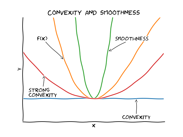
Definition (convexity). A differentiable function $f$ is said to be convex if for all $x,y \in \mathbb R^n$ it holds: $f(y) - f(x) \geq \langle \nabla f(x), y-x\rangle$.

Definition (smoothness). A convex function $f$ is said to be $L$-smooth if for all $x,y \in \mathbb R^n$ it holds: $f(y) - f(x) \leq \langle \nabla f(x), y-x\rangle + \frac{L}{2} \norm{x-y}^2$.

Definition (strong convexity). A convex function $f$ is said to be $\mu$-strongly convex if for all $x,y \in \mathbb R^n$ it holds: $f(y) - f(x) \geq \langle \nabla f(x), y-x\rangle + \frac{\mu}{2} \norm{x-y}^2$.

(Strong) convexity provides an underestimator of the function whereas smoothness provides an overestimator:

Convexity and smoothness

Now suppose that we consider (vanilla) gradient descent with updates of the form

\[\tag{GD} x_{t+1} \leftarrow x_t - \frac{1}{L} \nabla f(x_t).\]

Plugging-in this update into the definition of smoothness, we immediately obtain:

\[\tag{progress} \underbrace{f(x_{t}) - f(x_{t+1})}_{\text{primal progress}} \geq \frac{\norm{\nabla f(x_t)}^2}{2L}.\]

Similarly, with standard arguments we obtain from strong convexity the upper bound on the primal gap:

\[f(x_t) - f(x^\esx) \leq \frac{\norm{\nabla f(x_t)}^2}{2 \mu}.\]

We can now simply plug-in the upper bound into the progress inequality (progress) to obtain:

\[f(x_{t}) - f(x_{t+1}) \geq \frac{\norm{\nabla f(x_t)}^2}{2L} \geq \frac{\mu}{L} (f(x_t) - f(x^\esx)),\]

or, via rewriting,

\[f(x_{t+1}) - f(x^\esx) \leq \left(1- \frac{\mu}{L}\right) (f(x_t) - f(x^\esx)),\]

so that we obtain the coveted linear rate:

\[f(x_t) - f(x^\esx) \leq \left(1- \frac{\mu}{L}\right)^t (f(x_0) - f(x^\esx)).\]

While this is great, the best-known lower bound only rules out rates faster than $\Theta(\sqrt{\frac{\mu}{L}} \log \frac{1}{\varepsilon})$, so that we are potentially quadratically slower than the best possible. Acceleration closes this gap, achieving a convergence rate of $\Theta(\sqrt{\frac{\mu}{L}} \log \frac{1}{\varepsilon})$, which is optimal.

Information left on the table

A natural question to ask now is of course why gradient descent cannot achieve the optimal rate and whether it is a problem with the algorithm or the analysis (which is an important question one should ask routinely). For example, going from sublinear convergence in the case smooth and (non-strongly) convex function to linear convergence in the case of smooth and strongly convex function does not require any change in the algorithm, e.g., in (vanilla) gradient descent but rather it is a better analysis that establishes the better rate. A close examination of the argument from above shows that in each iteration $t+1$ we basically rely on two inequalities:

Smoothness at $x_t$:

\[f(y) - f(x_t) \leq \langle \nabla f(x_t), y-x_t\rangle + \frac{L}{2} \norm{x_t-y}^2.\]

Strong convexity at $x_t$:

\[f(y) - f(x_t) \geq \langle \nabla f(x_t), y-x_t\rangle + \frac{\mu}{2} \norm{x_t-y}^2.\]

The key point is that we use significantly less information than we actually have available: In fact, in iteration $t+1$, we have iterates $x_0, \dots, x_t$ and for each of them we have these two inequalities. In particular, we have the strong convexity lower bound for each $x_0, \dots, x_t$ potentially providing a much better lower approximation of $f$ than just the bound from the last iterate $x_t$. Roughly in picture world it looks like this, where the left is only using last-iterate information for the lower bound and the right is using all previous iterates:

MSC and SM inequalities

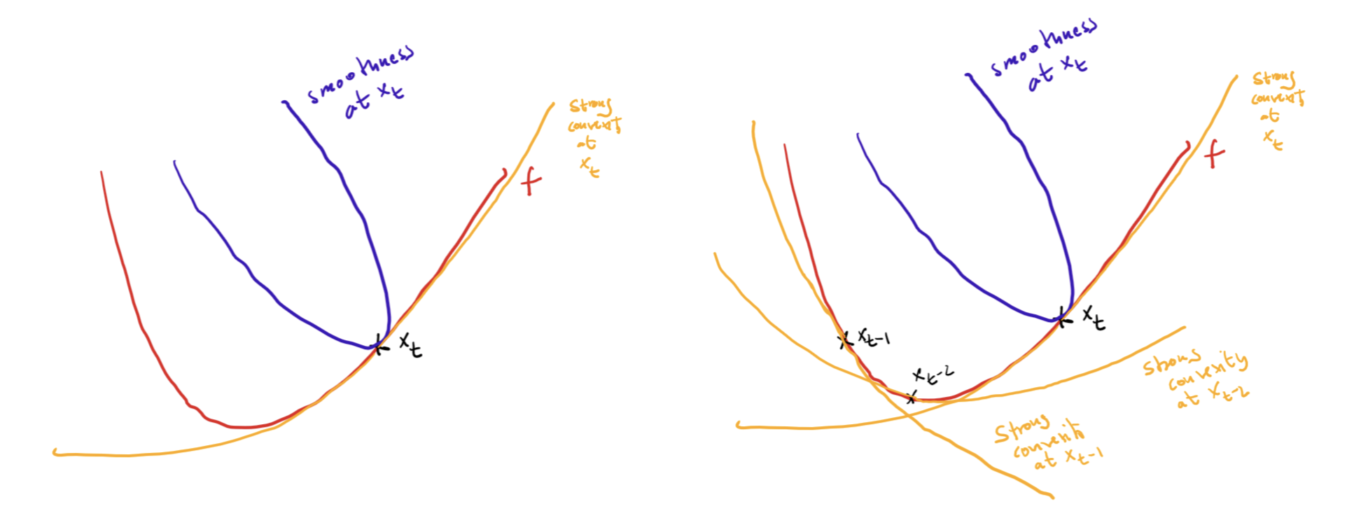
Can this additional information be used to improve convergence?

Acceleration

We will now try to derive our accelerated method. To this end assume that we already have a hypothetical algorithm that has generated iterates $y_0, \dots, y_t$ by some (as of now unknown) rule.

A better lower bound

Let us see whether we can use the additional information from previous iterates to obtain a better lower bound or approximation for our function. Given the sequence of iterates $y_0, \dots, y_t$ we have the following family of inequalities from strong convexity:

\[f(y_i) + \langle \nabla f(y_i), z - y_i \rangle + \frac{\mu}{2} \norm{y_i-z}^2 \leq f(z),\]

for $i \in \setb{0, \dots, t}$. Moreover we can take any positive combination of these inequalities with weights $a_0, \dots, a_t \geq 0$ and obtain:

\[\sum_{i = 0}^t a_i [f(y_i) + \langle \nabla f(y_i), z - y_i \rangle + \frac{\mu}{2} \norm{y_i-z}^2] \leq \underbrace{\left(\sum_{i = 0}^t a_i\right)}_{\doteq A_t} f(z),\]

or equivalently:

\[\frac{1}{A_t}\sum_{i = 0}^t a_i [f(y_i) + \langle \nabla f(y_i), z - y_i \rangle + \frac{\mu}{2} \norm{y_i-z}^2] \leq f(z).\]

This inequality holds for all $z \in \RR^n$ and in particular the optimal solution $x^\esx \in \RR^n$. We do not know $x^\esx$ however, but what we do know, taking the minimum over $z \in \RR^n$ on both sides, is the bound:

\[L_t \doteq \min_{z \in \RR^n} \frac{1}{A_t}\sum_{i = 0}^t a_i [f(y_i) + \langle \nabla f(y_i), z - y_i \rangle + \frac{\mu}{2} \norm{y_i-z}^2] \leq \min_{z \in \RR^n} f(z) = f(x^\esx).\]

Note that $L_t$ is a function of $a_0, \dots, a_t$ and $y_0, \dots, y_t$ and clearly the strength of the bound depends heavily on both; we will get back to both later. Next let us compute the minimizer of $L_k$. Clearly, $L_k$ is smooth and (strongly) convex in $z$ and the first-order optimality condition leads to the equation:

\[\begin{align*} 0 & = \frac{1}{A_t}\sum_{i = 0}^t a_i [\nabla f(y_i) - \mu (y_i - z) ] \\ & = \mu z + \frac{1}{A_t}\sum_{i = 0}^t a_i [\nabla f(y_i) - \mu y_i ] \\ \Leftrightarrow z &= \frac{1}{A_t}\sum_{i = 0}^t a_i [y_i - \frac{1}{\mu}\nabla f(y_i)], \end{align*}\]

so that the (dual) lower bound is optimized by

\[\tag{dualSeq} w_t \leftarrow \frac{1}{A_t}\sum_{i = 0}^t a_i [y_i - \frac{1}{\mu}\nabla f(y_i)],\]

which can also be written recursively using $A_t \doteq \sum_{i = 0}^t a_i$ as:

\[\tag{dualSeqRec} w_t \leftarrow \frac{A_{t-1}}{A_t} w_{t-1} + \frac{a_t}{A_t} [y_t - \frac{1}{\mu}\nabla f(y_t)].\]

Primal steps

For the primal steps we do exactly the same thing as before in gradient descent. After all, let us first see how far we can get with only adjusting the lower bound. Therefore, given the sequence $y_0, \dots, y_t$ in iteration $t$, we define the primal steps as

\[\tag{primalSeq} x_t \leftarrow y_t - \frac{1}{L} \nabla f(y_t),\]

which is the same update as in (GD) but we do not use the update to (directly) define the next iterates $y_{t+1}$ but rather let us give them a different name until we decide what to do with them.

Interlude: Approximate Dual Gap Technique (ADGT)

Having now a (hopefully) better lower bound we need to see what we can do with it. For this we will use the Approximate Dual Gap Technique (ADGT) of [DO], a conceptually simple yet powerful technique to analyze first-order methods. In a nutshell, ADGT works as follows: Our ultimate aim is to prove that for some first-order algorithm that generates iterates $x_0, \dots, x_t, \dots$ the optimality gap $f(x_t) - f(x^\esx) \rightarrow 0$ with a certain convergence rate. Usually, it is very hard to say something about $f(x_t) - f(x^\esx)$ directly and so typically analyses use bounds on the optimality gap.

ADGT makes this explicit in a first step by working with a lower bound $L_t \leq f(x^\esx)$ in iteration $t$ and upper bound $f(x_t) \leq U_t$ and then defining a gap estimate in iteration $t$ as $G_t \doteq U_t - L_t$, so that $f(x_t) - f(x^\esx) \leq G_t$ in each iteration $t$. Then further, if there exists a sequence of suitably chosen, fast growing numbers $0 \leq A_0, \dots, A_t, \dots$, so that

\[A_t G_t \leq A_{t-1} G_{t-1}.\]

Then in particular the gap estimate in iteration $t$ drops as $G_t \leq \frac{A_{t-1}}{A_t} G_{t-1}$ and after chaining these bounds together we obtain $f(x_t) - f(x^*) \leq \frac{A_0}{A_t} G_0$, i.e., the convergence rate is given basically by $\frac{1}{A_t}$.

Before going back to our attempt at acceleration, let us familiarize ourselves with ADGT by analyzing vanilla gradient descent with update (GD). To this end let us consider a simplified and stronger lower bound, given by

\[\hat L_t \doteq \frac{1}{A_t} \sum_{i = 0}^t a_i [f(x_i) + \langle \nabla f(x_i), x^\esx - x_i \rangle + \frac{\mu}{2} \norm{x_i-x^\esx}^2] \leq f(x^\esx),\]

where we chose $z = x^\esx$ with $A_t \doteq \sum_{i = 0}^t a_i$, so that we only have to pick the $a_i$ at some point. For the upper bound we simple choose $U_t \doteq f(x_{t+1})$; mind the index shift as it will be important.

In order to show that $A_t G_t \leq A_{t-1} G_{t-1}$, we will analyze the upper bound change and the lower bound change separately as our goal is to show:

\[0 \geq A_t G_t - A_{t-1} G_{t-1} = A_t U_t - A_{t-1} U_{t-1} - (A_t L_t - A_{t-1} L_{t-1}).\]

Change in upper bound.
The change in the upper bound can be bounded using smoothness with basically the same argument as for the vanilla GD warmup from above:

\[\begin{align*} A_t U_t - A_{t-1} U_{t-1} & = A_t f(x_{t+1}) - A_{t-1} f(x_{t}) = A_t (f(x_{t+1}) - f(x_{t})) + a_t f(x_{t}) \\ & \leq - A_t \left(\frac{\norm{\nabla f(x_{t})}^2}{2L}\right) + a_t f(x_{t}). \end{align*}\]

Change in lower bound.
The change in the lower bound follows from evaluating $\hat L_t$, which used the strong convexity of $f$ in its definition:

\[\begin{align*} A_t \hat L_t - A_{t-1} \hat L_{t-1} & = a_t [f(x_t) + \langle \nabla f(x_t), x^\esx - x_t \rangle + \frac{\mu}{2} \norm{x_t-x^\esx}^2] \end{align*}\]

Change in the gap estimate.
With this we immediately obtain that the change in the gap estimate is given by:

\[\begin{align*} A_t G_t - A_{t-1} G_{t-1} & \leq a_t (\underbrace{f(x_{t}) - f(x_t)}_{= 0}) - A_t \left(\frac{\norm{\nabla f(x_{t})}^2}{2L}\right) - a_t [\langle \nabla f(x_t), x^\esx - x_t \rangle + \frac{\mu}{2} \norm{x_t-x^\esx}^2] \\ & \leq - A_t \left(\frac{\norm{\nabla f(x_{t})}^2}{2L}\right) - \frac{a_t}{2\mu} [\underbrace{2\mu \langle \nabla f(x_t), x^\esx - x_t \rangle + \mu^2 \norm{x_t-x^\esx}^2}_{\geq - \norm{ \nabla f(x_t)}^2 \text{ via } a^2 + 2ab \geq - b^2}] \\ & \leq \norm{\nabla f(x_{t})}^2 \left( - \frac{A_t}{2L} + \frac{a_t}{2\mu} \right), \end{align*}\]

using the standard trick $a^2 + 2ab \geq - b^2$ that virtually every proof utilizing strong convexity uses (see Cheat Sheet: Frank-Wolfe and Conditional Gradients for a derivation of that estimation). Thus for

\[A_t G_t - A_{t-1} G_{t-1} \leq 0,\]

it suffices to choose $a_t$, so that $- \frac{A_t}{2L} + \frac{a_t}{2\mu} \leq 0$ and the choice $\frac{a_t}{A_t} \doteq \frac{\mu}{L}$ suffices, leading to a contraction with rate:

\[\frac{A_{t-1}}{A_t} = 1 - \frac{a_t}{A_t} = 1 - \frac{\mu}{L},\]

which is the standard rate and matches what we have derived above in the warmup. In a last step one would now relate $G_0$ to the initial gap $f(x_0) - f(x^\esx)$ to obtain a bound on the constant $A_0$. We skip this step to keep the exposition clean; it is immediate here and as it is not that crucial for our discussion.

Now is a good time to pause for a second. Initially we speculated that maybe not using all available information might be the reason for not obtaining a better rate. Yet, in this argument now, we have used more information, in fact in iteration $t$ we have used all iterates $x_0, \dots, x_{t-1}$; see definition of $\hat L_t$. Maybe this is because the iterates $x_t$ are obtained without any regard for the lower bound and while we use all iterates now, maybe the bound is not much stronger than the bound arising from the last iterate and maybe we could strengthen it by a better choice of the $a_i$ and $y_i$ in the general definition of $L_t$?

ADGT on the hypothetical sequence

While ADGT seems to be an overkill for the standard linear convergence proof compared to the argument from the warmup, we will see soon that ADGT buys us considerable extra freedom. We will now try to apply the same analysis as above once more however, we start out with our hypothetical sequence $y_0, \dots, y_t, \dots$ and see, whether maybe naturally a way arises to choose the $y_t$ not only to produce primal progress as the rule (GD) does but also dual progress, improving our lower bound estimate by providing better “attachment points” $y_0, \dots, y_t$ from which we obtain a stronger lower bound $L_t$ via strong convexity.

Observe that, given the sequence of iterates $y_0, \dots, y_t$, our primal iterates $x_t$ and dual iterates $w_t$ are the optimal updates in iteration $t$ for primal and dual progress respectively. Note, that in general we do not know whether $w_t = x_t$ and usually they are not equal.

We follow the same strategy as above with the aim of analyzing the change in the gap estimate for our partially specified algorithm:

Change in upper bound.
The change in the upper bound can be bounded using smoothness but applied to the update $x_t \leftarrow y_t - \frac{1}{L} \nabla f(y_t)$ that we used to define our primal sequence $x_t$, i.e., $f(x_t) - f(y_t) \leq - \frac{\norm{\nabla f(y_t)}^2}{2L}$. Otherwise, except for rearranging, using the upper bound $U_t \doteq f(x_{t})$ and adding zero it is the same; note the index shift from $t+1$ to $t$ in the definition of $U_t$ as we have the intermediate point $y_t$ now as will become clear:

\[\begin{align*} A_t U_t - A_{t-1} U_{t-1} & = A_t f(x_t) - A_{t-1} f(x_{t-1}) \\ & = A_t f(y_t) - A_t f(y_t) + A_t f(x_t) - A_{t-1} f(x_{t-1}) \\ & = a_t f(y_t) + A_t (f(x_t) - f(y_t)) + A_{t-1} (f(y_{t}) - f(x_{t-1})) \\ & \leq a_t f(y_t) - A_t \left(\frac{\norm{\nabla f(y_t)}^2}{2L}\right) + A_{t-1} (f(y_{t}) - f(x_{t-1})). \end{align*}\]

Change in lower bound.
The change in the lower bound this time around is more intricate however as we now have an optimization problem in the definition of $L_k$ that defines the dual iterates $w_t$. Recall that:

\[\begin{align*} L_t & = \min_{z \in \RR^n} \frac{1}{A_t}\sum_{i = 0}^t a_i [f(y_i) + \langle \nabla f(y_i), z - y_i \rangle + \frac{\mu}{2} \norm{y_i-z}^2] \\ & = \frac{1}{A_t}\sum_{i = 0}^t a_i f(y_i) + \frac{1}{A_t}\min_{z \in \RR^n} \underbrace{\sum_{i = 0}^t a_i [\langle \nabla f(y_i), z - y_i \rangle + \frac{\mu}{2} \norm{y_i-z}^2]}_{\doteq \gamma_t(z)}. \end{align*}\]

With this we can conveniently express the change in the lower bound as:

\[\begin{align*} A_t L_t - A_{t-1} L_{t-1} & = a_t f(y_t) + \gamma_t(w_t) - \gamma_{t-1}(w_{t-1}), \end{align*}\]

so that it suffices to bound the change $\gamma_t(w_t) - \gamma_{t-1}(w_{t-1})$. We have:

\[\begin{align*} \gamma_t(w_t) - \gamma_{t-1}(w_{t-1}) & = \gamma_{t-1}(w_{t}) + a_t \langle \nabla f(y_t), w_{t} - y_t \rangle + a_t\frac{\mu}{2} \norm{y_t-w_{t}}^2 - \gamma_{t-1}(w_{t-1}) \\ & = \gamma_{t-1}(w_{t-1}) + \underbrace{\langle \nabla \gamma_{t-1}(w_{t-1}), w_{t} - w_{t-1}\rangle}_{= 0\text{, as $w_{t-1}$ is a minimizer of $\gamma_{t-1}$}} + \frac{\mu A_{t-1}}{2} \norm{w_t - w_{t-1}}^2 \\ & \qquad \qquad + a_t \langle \nabla f(y_t), w_{t} - y_t \rangle + a_t \frac{\mu}{2} \norm{y_t-w_{t}}^2 - \gamma_{t-1}(w_{t-1}) \\ & = a_t \langle \nabla f(y_t), w_{t} - y_t \rangle + \frac{A_t\mu}{2}\left(\frac{A_{t-1}}{A_t} \norm{w_t - w_{t-1}}^2 + \frac{a_t}{A_t} \norm{y_t-w_{t}}^2 \right) \\ & \geq a_t \langle \nabla f(y_t), w_{t} - y_t \rangle + \frac{A_t \mu}{2} \norm{w_t - \frac{A_{t-1}}{A_t} w_{t-1} - \frac{a_t}{A_t} y_t}^2 \\ & = a_t \langle \nabla f(y_t), w_{t} - y_t \rangle + \frac{A_t \mu}{2} \norm{\frac{a_t}{A_t} \frac{1}{\mu}\nabla f(y_t)}^2, \end{align*}\]

where the second equation is by the Taylor expansion of $\gamma_{t-1}$ around $w_{t-1}$ evaluated at $w_t$, the first inequality is by Jensen’s inequality, and the fourth equation is by the recursive definition (dualSeqRec) of $w_t$. With this we obtain that the change is in the lower bound can be bounded as:

\[A_t L_t - A_{t-1} L_{t-1} \geq a_t f(y_t) + a_t \langle \nabla f(y_t), w_{t} - y_t \rangle + \frac{A_t \mu}{2} \norm{\frac{a_t}{A_t} \frac{1}{\mu}\nabla f(y_t)}^2.\]

Change in the gap estimate.
With the above, we can now bound the change in the gap estimate, where the inequality is by convexity, via:

\[\begin{align*} A_t G_t - A_{t-1} G_{t-1} & \leq a_t f(y_t) - A_t \left(\frac{\norm{\nabla f(y_t)}^2}{2L}\right) + A_{t-1} (f(y_{t}) - f(x_{t-1})) - a_t f(y_t) \\ & \qquad \qquad - a_t \langle \nabla f(y_t), w_{t} - y_t \rangle - \frac{A_t \mu}{2} \norm{\frac{a_t}{A_t} \frac{1}{\mu}\nabla f(y_t)}^2 \\ & = - A_t \left(\frac{\norm{\nabla f(y_t)}^2}{2L} + \frac{a_t^2}{A_t^2} \frac{\norm{\nabla f(y_t)}^2}{2\mu} \right) + A_{t-1} (f(y_{t}) - f(x_{t-1})) - a_t \langle \nabla f(y_t), w_{t} - y_t \rangle \\ & \leq - A_t \left(\frac{\norm{\nabla f(y_t)}^2}{2L} + \frac{a_t^2}{A_t^2} \frac{\norm{\nabla f(y_t)}^2}{2\mu} \right) + A_{t-1} \langle \nabla f(y_t), y_{t} - x_{t-1} \rangle - a_t \langle \nabla f(y_t), w_{t} - y_t \rangle \\ & = - A_t \left(\frac{\norm{\nabla f(y_t)}^2}{2L} + \frac{a_t^2}{A_t^2} \frac{\norm{\nabla f(y_t)}^2}{2\mu} \right) + \langle \nabla f(y_t), A_t y_{t} - A_{t-1} x_{t-1} - a_t w_t \rangle. \end{align*}\]

While maybe a little tedious, so far nothing special has happened. We simply computed the change in the gap estimate via the change in the upper bound and the change in the lower bound. Now we need the right-hand side to be non-positive to complete the proof and derive the rate. Our goal is to show:

\[\tag{gapCondition} - A_t \left(\frac{\norm{\nabla f(y_t)}^2}{2L} + \frac{a_t^2}{A_t^2} \frac{\norm{\nabla f(y_t)}^2}{2\mu} \right) + \langle \nabla f(y_t), A_t y_{t} - A_{t-1} x_{t-1} - a_t w_t \rangle \leq 0,\]

which we would obtain, dividing by $A_t$ and defining $\tau \doteq \frac{a_t}{A_t}$, if we can ensure:

\[\tag{impY} y_{t} - (1-\tau) x_{t-1} - \tau w_t = \nabla f(y_t) \left(\frac{1}{2L} + \tau^2 \frac{1}{2\mu} \right),\]

as then the left hand side in (gapCondition) evaluates to $0$. Note that (impY) almost provides a definition of the $y_t$, which is our last missing piece but not quite: the $w_t$ depends itself on $y_t$ and we would rather have it an explicit function of $w_{t-1}$. Luckily we have the recursive definition of the $w_t$ from (dualSeqRec) that will allow us to unroll one step:

\[\begin{align*} \nabla f(y_t) \left(\frac{1}{2L} + \tau^2 \frac{1}{2\mu} \right) & = y_{t} - (1-\tau) x_{t-1} - \tau w_t \\ & = y_t - (1-\tau) x_{t-1} - \tau (1-\tau) w_{t-1} - \tau^2 (y_t - \frac{1}{\mu} \nabla f(y_t)). \end{align*}\]

After rearranging, the above becomes:

\[\tag{expY} \nabla f(y_t) \left(\frac{1}{2L} - \tau^2 \frac{1}{2\mu} \right) = (1-\tau^2) y_t - (1-\tau) x_{t-1} - \tau (1-\tau) w_{t-1},\]

and we are free to make some choices. For $\tau = \frac{a_t}{A_t} \doteq \sqrt{\frac{\mu}{L}}$, the left-hand side becomes $0$ and after dividing by $(1-\tau)$, we obtain:

\[(1+\tau) y_t = x_{t-1} + \tau w_{t-1},\]

which finally provides the desired definition of the $y_t$ and, recalling that we contract at a rate of $1-\frac{a_t}{A_t}$, we achieve a contraction of the gap at a rate of $1-\frac{a_t}{A_t} = 1-\tau = 1 - \sqrt{\frac{\mu}{L}}$ as required:

\[\tag{accRate} f(x_t) - f(x^\esx) \leq \left(1 - \sqrt{\frac{\mu}{L}}\right)^t (f(x_0) - f(x^\esx)).\] \[\qed\]

This completes our argument. Now that we are done with this exercise it is time to pause and recap. First, let us state the full algorithm; we only output the primal sequence $x_1, \dots, x_t, \dots$ here but the other sequences are useful as well:

Algorithm. (Accelerated Gradient Descent)
Input: $L$-smooth and $\mu$-strongly convex function $f$. Initial point $x_0$.
Output: Sequence of iterates $x_0, \dots, x_t$
$w_0 \leftarrow x_0$
$\tau \leftarrow \sqrt{\frac{\mu}{L}}$
For $t = 1, \dots, t$ do
$\qquad$ $y_t \leftarrow \frac{1}{1 + \tau} x_{t-1} + \frac{\tau}{1 + \tau} w_{t-1} \qquad \text{{update mixing sequence $y_t$}}$
$\qquad$ $w_t \leftarrow (1-\tau) w_{t-1} + \tau (y_t - \frac{1}{\mu} \nabla f(y_t)) \qquad \text{{update dual sequence $w_t$}}$
$\qquad$ $x_t \leftarrow y_t - \frac{1}{L} \nabla f(y_t)\qquad \text{{update primal sequence $x_t$}}$

Next, a few remarks are in order:

Remarks.

What the analysis shows is that acceleration is achieved by simultaneously optimizing the primal and dual, i.e., upper and lower bound on the gap. This is in contrast to vanilla gradient descent that first and foremost maximizes primal progress per iteration and not gap closed per iteration. The key here is the definition of the sequence $y_t$ that balances primal and dual progress and ensures optimal progress in gap closed per iteration. Moreover, it is important to note that this is not simply a better analysis of the same algorithm but rather the iterates in the algorithm do really differ from gradient descent and acceleration really materializes in faster convergence rates; see computations below.
The $y_t$ are chosen to be a convex combination of the primal and the dual step. This combination is formed with fixed weights that do not change across the algorithm’s progression.
The proof establishes that in each iteration we contract the gap by a multiplicative factor $(1-\tau)$. It is neither guaranteed that we make primal progress per iteration nor that we make dual progress in each iteration. What is guaranteed is that the in sum we make enough progress; we will get back to this further below.
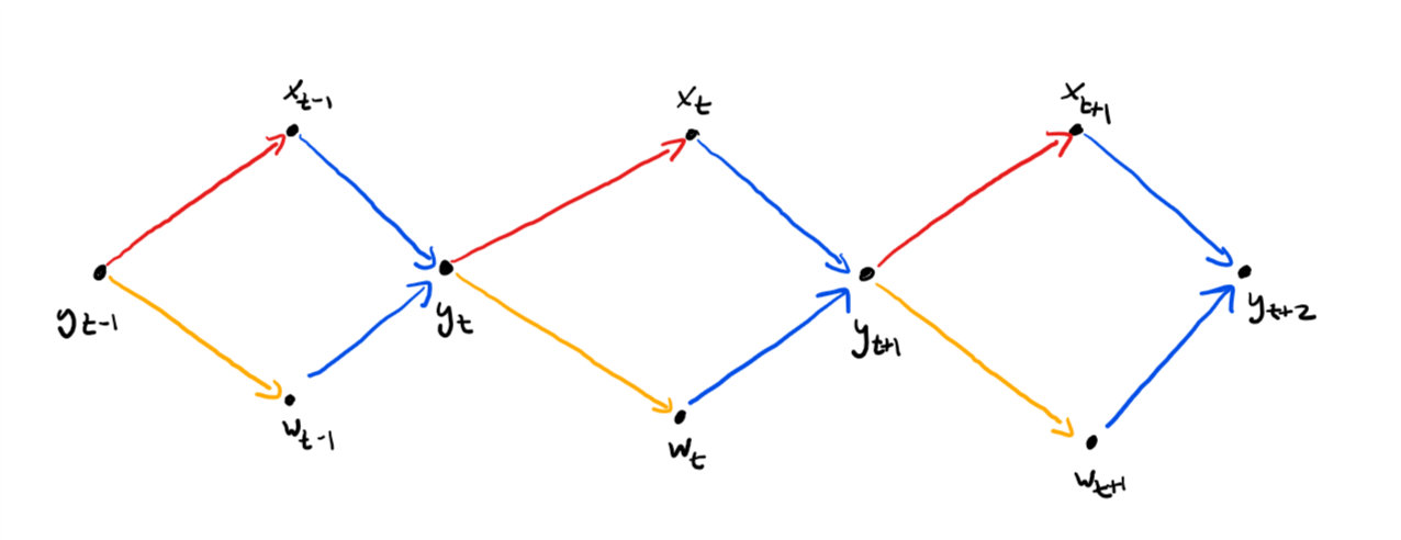
The primal and dual iterates in iteration $k$ are independent of each other conditioned on the $y_k, \dots, y_0$; see the graphics below. This is quite helpful for modifications as we will see in the next section.

Information Flow Acceleration

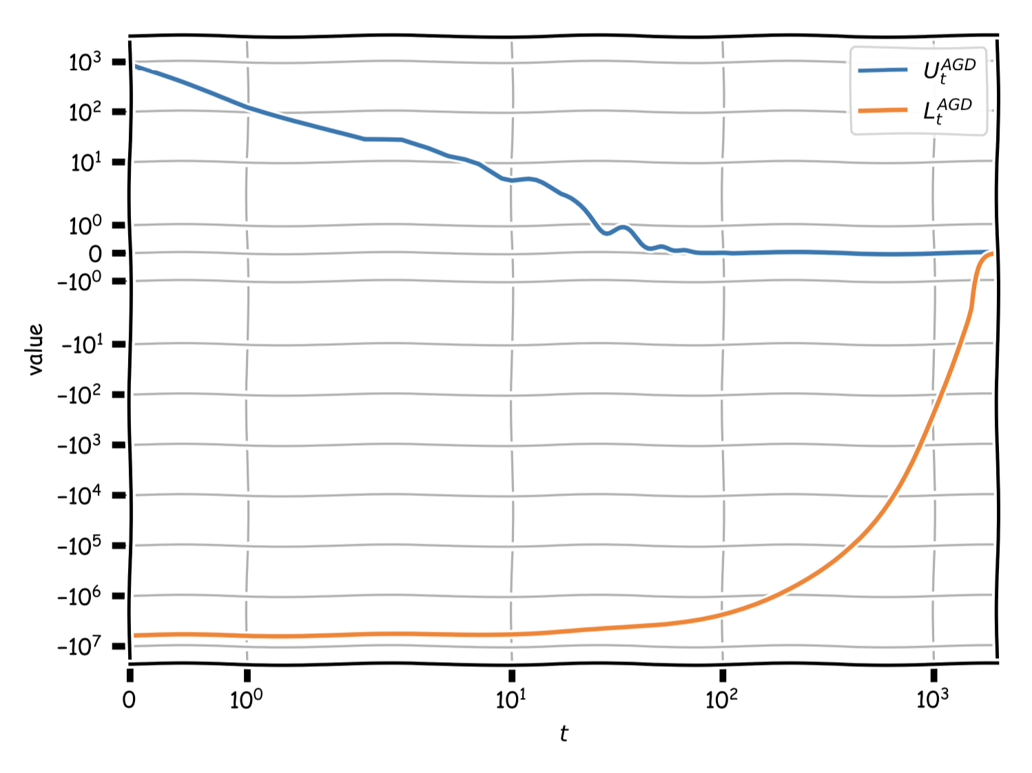
We will now compare the method from above to vanilla gradient descent. The instance that we consider is a quadratic with condition number $\theta = \frac{\mu}{L} = 10000$ in $\RR^n$, where $n = 100$. We run the algorithms for $2000$ iterations.

The first figure shows the gap evolution of $U_t$ and $L_t$ across iterations for the accelerated method. It can be seen that indeed the upper bound $U_t$, which is given by the primal function value, is not necessarily monotonic as compared to e.g., gradient descent. The plot is in log-log scale to better visualize behavior.

Gap evolution

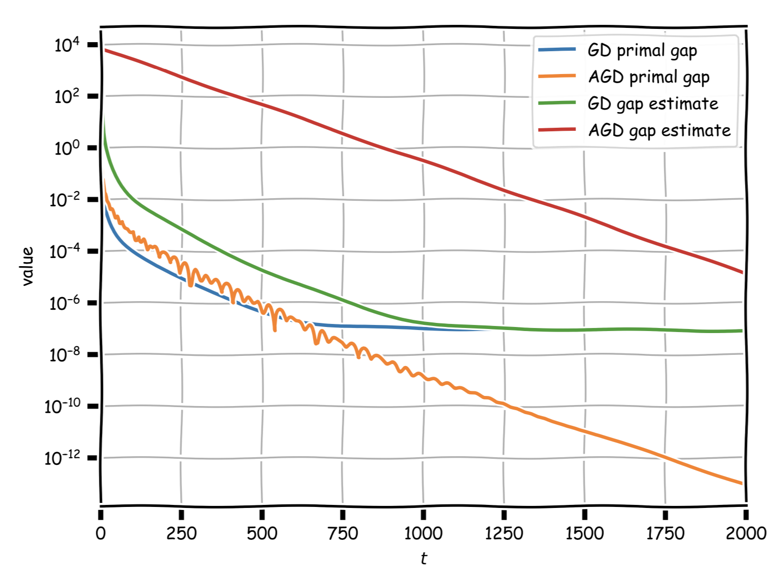
The next figure compares vanilla gradient descent (GD) vs. our accelerated method (AGD) with respect to the (true) primal gap as well as the gap estimate $G_t$. It can be seen that the convergence rate of AGD is much higher than the rate of GD. Note that GD is not converging prematurely but the rate is significantly lower. While the AGD gap estimate has a much higher offset, it contracts basically at the same rate as the (true) primal gap.

GD vs. AGD

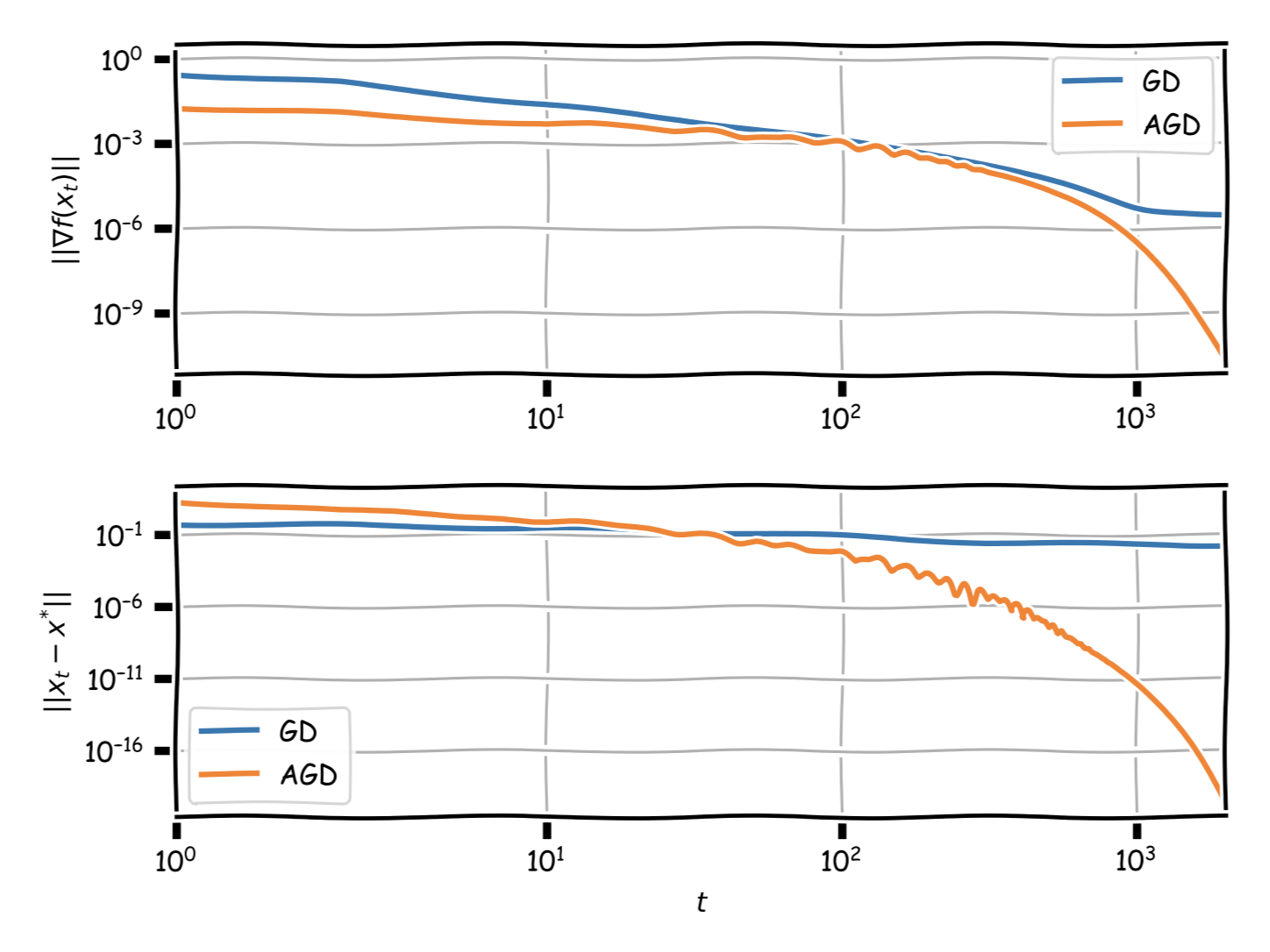
Finally, the last figure depicts the evolution of the distance to the optimal solution as well as the norm of the gradient (both optimality measures) for GD and AGD. Note that while these measures are not monotonic for AGD, they converge much faster.

Auxiliary Measures

Extensions

We will now briefly discuss extensions of the argumentation from above.

Monotonic variant

The presented argument above is for the most basic case and as mentioned in the remarks usually the primal gap is not monotonously decreasing. This can be an issue in some cases. In the following we discuss a modification of the above to ensure monotonous primal progress, which, by strong convexity, also ensures monotonous decrease in distance to the optimal solution. Such modifications are reasonably well-known, e.g., Nesterov used it to define an accelerated method that ensures monotonous progress in the distance to the optimal solution. Here we will see that such modifications are easily handled in the ADGT framework.

In order to achieve the above we will actually prove something stronger: we show that we can mix-in an auxiliary sequence of points $\tilde x_1, \dots, \tilde x_t, \dots$ and the algorithm will choose the better of the two (in terms of function value) between the provided point and the accelerated step. Then it suffices to, e.g., choose the sequence $\tilde x_1, \dots, \tilde x_t, \dots$ to be standard gradient steps $\tilde x_t \leftarrow x_{t-1} - \frac{1}{L} \nabla f(x_{t-1})$ to obtain a monotonic variant.

Algorithm. (Accelerated Gradient Descent with mixed-in sequence)
Input: $L$-smooth and $\mu$-strongly convex function $f$. Initial point $x_0$. Sequence $\tilde x_1, \dots, \tilde x_t, \dots$.
Output: Sequence of iterates $x_0, \dots, x_t$
$w_0 \leftarrow x_0$
$\tau \leftarrow \sqrt{\frac{\mu}{L}}$
For $t = 1, \dots, t$ do
$\qquad$ $y_t \leftarrow \frac{1}{1 + \tau} x_{t-1} + \frac{\tau}{1 + \tau} w_{t-1} \qquad \text{{update mixing sequence $y_t$}}$
$\qquad$ $w_t \leftarrow (1-\tau) w_{t-1} + \tau (y_t - \frac{1}{\mu} \nabla f(y_t)) \qquad \text{{update dual sequence $w_t$}}$
$\qquad$ $\bar x_t \leftarrow y_t - \frac{1}{L} \nabla f(y_t)\qquad \text{{update primal sequence $x_t$}}$
$\qquad$ $x_t \leftarrow \arg\min \setb{f(\bar x_t), f(\tilde x_t)}\qquad \text{{take better point}}$

At first this might seem problematic as we argued before, that it is the intricate construction of the $y_t$ that simultaneously optimize the primal upper and lower bound. In fact, we potentially sacrificed primal progress (the method is not monotonic anymore after all) to close the gap faster. Now that we play around with the definition of the $x_t$ (and in turn with the $y_t$) in such a heavy-handed way we might break acceleration. It turns out however that the above works just fine. To see this let us redo the analysis. First of all, note that for a given $y_t$ the analysis of the lower bound improvement remains the same as there is no dependence on $x_{t-1}$ given $y_t$. So let us re-examine the upper bound:

Change in upper bound.
It suffices to observe that $f(x_t) \leq f(\bar x_t)$ and hence the change in the upper bound can be bounded as before using $\bar x_t \leftarrow y_t - \nabla f(y_t)$ which implies $f(\bar x_t) - f(y_t) \leq - \frac{\norm{\nabla f(y_t)}^2}{2L}$:

\[\begin{align*} A_t U_t - A_{t-1} U_{t-1} & = A_t f(x_t) - A_{t-1} f(x_{t-1}) \leq A_t f(\bar x_t) - A_{t-1} f(x_{t-1}) \\ & = A_t f(y_t) - A_t f(y_t) + A_t f(\bar x_t) - A_{t-1} f(x_{t-1}) \\ & = a_t f(y_t) + A_t (f(\bar x_t) - f(y_t)) + A_{t-1} (f(y_{t}) - f(x_{t-1})) \\ & \leq a_t f(y_t) - A_t \left(\frac{\norm{\nabla f(y_t)}^2}{2L}\right) + A_{t-1} (f(y_{t}) - f(x_{t-1})). \end{align*}\]

Thus we obtain an identical bound for the change in the upper bound. Not really surprising as we potentially only do better due to the auxiliary sequence. Now it remains to derive the definition of the $y_t$ from $x_{t-1}$ and $w_{t-1}$.

Change in the gap estimate.
The first part of the estimation is a direct combination of the upper bound estimate and the lower bound estimate. Note that the definition of the $y_t$ depended on $x_{t-1}$ and $w_{t-1}$ before and we have to carefully check the impact of the changed definition of $x_{t-1}$. The manipulations combining the upper and the lower bound estimate however do not make special use of how $x_{t-1}$ is defined and we similarly end up with:

as before and the goal is again to choose $y_t$ to ensure the above is satisfied. With the same computations as before we obtain with $\tau \doteq \frac{a_t}{A_t} \doteq \sqrt{\frac{\mu}{L}}$:

\[\tag{expY} \nabla f(y_t) \left(\frac{1}{2L} - \tau^2 \frac{1}{2\mu} \right) = (1-\tau^2) y_t - (1-\tau) x_{t-1} - \tau (1-\tau) w_{t-1}.\]

and plugging in the value of $\tau$ and rearranging leads to:

\[(1+\tau) y_t = x_{t-1} + \tau w_{t-1},\]

and the conclusion follows as before. The key point here is that also these estimations do not rely on the specific form of $x_{t-1}$. The only thing that we really needed and where the definition of the $x_{t-1}$ played a role is that we make enough progress in terms of the upper bound estimate. Basically, we can define $y_t$ from any $x_{t-1}$ and $w_{t-1}$ as long as they satisfy the upper bound and lower bound estimates.

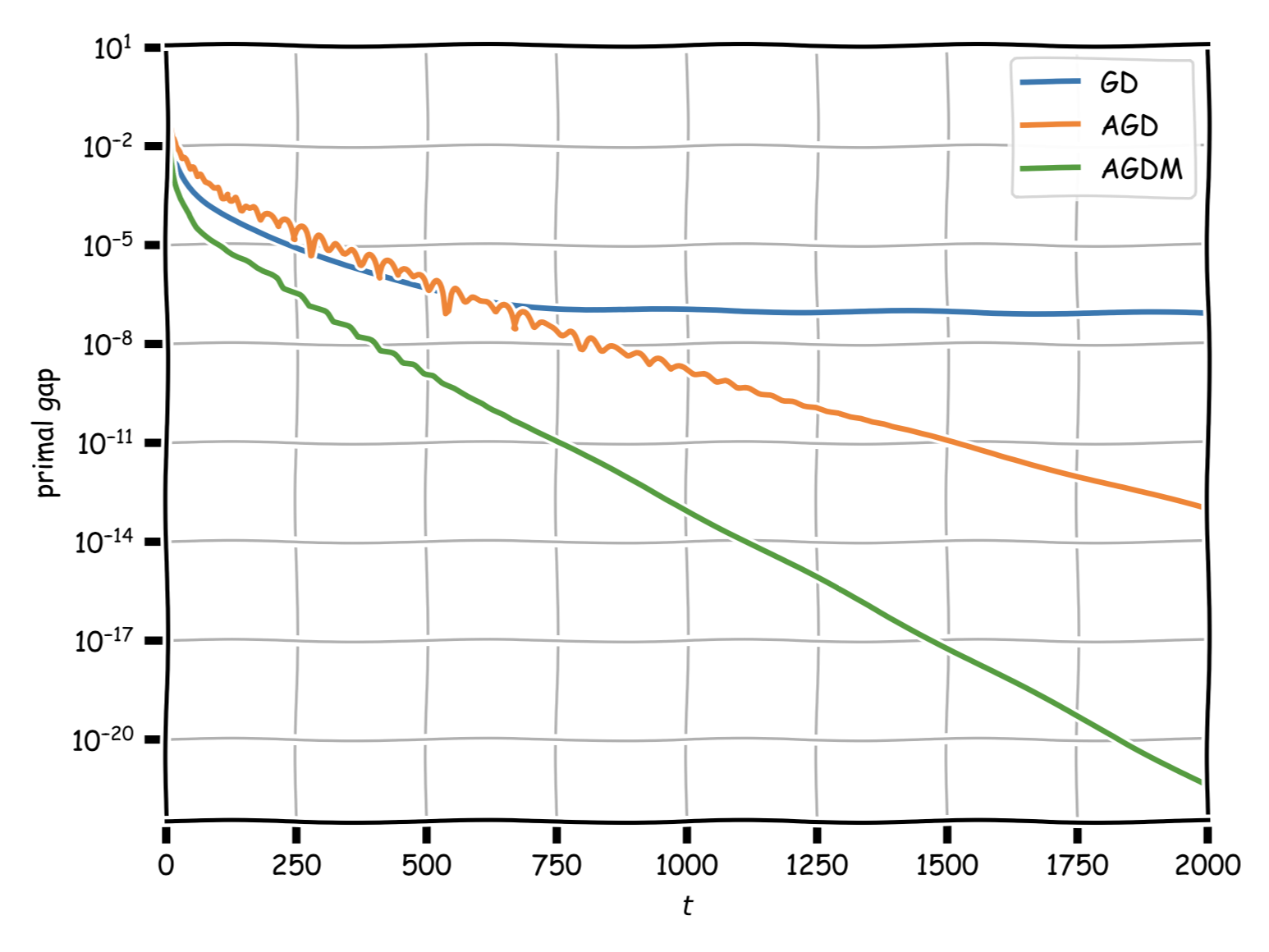
The following figure compares the monotonic variant of the accelerated method (AGDM) to the non-monotonic accelerated method (AGD) and vanilla gradient descent (GD) in terms of primal gap evolution. Observe that AGDM is not just monotonic but also has an (empirically) higher convergence rate. The instance is the same as above:

Monotonic

The smooth and (non-strongly) convex case

It is known that in the smooth and (non-strongly) convex case acceleration is also possible, improving from $O(1/t)$ (or equivalently $O(1/\varepsilon)$) convergence to $O(1/t^2)$ (or equivalently $O(1/\sqrt{\varepsilon})$) convergence. We could establish this result with the analysis from above, by adjusting the lower bound $L_t$ to not rely on strong convexity but convexity only. However, the resulting lower bound is not going to be smooth anymore, so that the simple trick of optimizing out the bound we used above is not going to work anymore. The answer to this is a more complicated (but natural) smoothening of the lower bound function and the interested reader is referred to [DO]. There is another way however, that essentially achieves the same result, up to log-factors, and leverages what we have proven already. We replicate the argument from [SAB] here.

The basic idea is that we take our smooth function $f$ and given an accuracy $\varepsilon$, we mix in a weak quadratic to make the function strongly convex and then we run the algorithm from above.

Let $f$ be $L$-smooth and assume that $x_0$, our initial iterate, is close enough to the optimal solution so that $D \doteq \norm{x_0 - x^\esx} \geq \norm{x_t - x^\esx}$ for all $t$; the “burn-in” until we reach such a point happens after at most a finite number of iterations, independent of $\varepsilon$. Given a target accuracy $\varepsilon > 0$, we simply define:

\[f_\varepsilon(x) \doteq f(x) + \frac{\varepsilon}{2D^2} \norm{x_0 - x}^2.\]

Observe that $f_\varepsilon$ is now $(L + \frac{\varepsilon}{2D^2})$-smooth and $\frac{\varepsilon}{2D^2}$-strongly convex. Moreover, essentially minimizing $f_\varepsilon$ is the same a minimizing $f$ up to small error:

\[\begin{align*} f(x_t) - f(x^\esx) & = f_\varepsilon(x_t) - \frac{\varepsilon}{2D^2} \norm{x_0 - x_t}^2 - f_\varepsilon(x^\esx) + \frac{\varepsilon}{2D^2} \norm{x_0 - x^\esx}^2 \\ & \leq f_\varepsilon(x_t) - f_\varepsilon(x^\esx) + \frac{\varepsilon}{2} \leq f_\varepsilon(x_t) - f_\varepsilon(x_\varepsilon^\esx) + \frac{\varepsilon}{2}, \end{align*}\]

where $x_\varepsilon^\esx$ is the optimal solution to $\min_{x} f_\varepsilon(x)$. This shows finding an $\varepsilon/2$-optimal solution $x_t$ to $\min_{x} f_\varepsilon(x)$ provides an $\varepsilon$-optimal solution to $\min_x f(x)$.

Now we run the accelerated method from above on $f_\varepsilon$ with accuracy $\varepsilon/2$. We had an accelerated rate (accRate) of

\[f(x_t) - f(x^\esx) \leq \left(1 - \sqrt{\frac{\mu}{L}}\right)^t (f(x_0) - f(x^\esx)),\]

for a generic $L$-smooth and $\mu$-strongly convex function $f$. Moreover, $f_\varepsilon(x_0) - f_\varepsilon(x^\esx) \leq \frac{(L+\varepsilon)D^2}{2}$ by smoothness. We now simply plug-in parameters and obtain:

\[f_\varepsilon(x_t) - f_\varepsilon(x^\esx) \leq \left(1 - \sqrt{\frac{\frac{\varepsilon}{2D^2}}{L + \frac{\varepsilon}{2D^2}}}\right)^t \left(\frac{(L+\varepsilon)D^2}{2}\right),\]

so that in order to achieve $f_\varepsilon(x_t) - f_\varepsilon(x^\esx) \leq \varepsilon/2$ it suffices to satisfy:

\[\begin{align*} t \log \left(1 - \sqrt{\frac{\frac{\varepsilon}{2D^2}}{L + \frac{\varepsilon}{2D^2}}}\right) & \leq - \log \frac{(L+\varepsilon)D^2}{2} + \log \frac{\varepsilon}{2} \\ \Leftrightarrow t & \geq - \frac{\log \frac{(L+\varepsilon)D^2}{\varepsilon} }{\log \left(1 - \sqrt{\frac{\frac{\varepsilon}{2D^2}}{L + \frac{\varepsilon}{2D^2}}}\right)}, \end{align*}\]

and using $\log 1-r \approx - r$ for $r$ small and $L + \frac{\varepsilon}{2D^2} \approx L$ we obtain that in order to ensure $f(x_t) - f(x^\esx) \leq \varepsilon$, we need to run the accelerated method on the smooth function $f_\varepsilon$ for roughly no more than:

\[t \approx \log \left(\frac{(L+\varepsilon)D^2}{\varepsilon} \right) \sqrt{\frac{2LD^2}{\varepsilon}},\]

iterations. This matches, up to a logarithmic term, the complexity that we would expect from an accelerated method in the smooth (non-strongly) convex case.

Acceleration and noise

One of the often-cited major drawbacks of accelerated methods is that they do not deal well with noisy or inexact gradients, i.e, they are not robust. To make matters worse, in [DGN] it was shown that basically any method that is faster than vanilla Gradient Descent necessarily needs to accumulate errors linearly in the number of iterations. This poses significant challenges depending on the magnitude of the noise. Slightly cheating here and considering the smooth and (non-stronlgy) convex case (check out [DGN] and Moritz’s post on Robustness vs. Acceleration for precise definitions and some nice computations), suppose that the magnitude of error in the gradients is $\delta$, then vanilla Gradient Descent after $t$ iterations provides a solution with guarantee:

\[f(x_t) - f(x^\esx) \leq O(1/t) + \delta,\]

whereas Accelerated Gradient Descent (the standard one, see [DGN]) provides a solution that satisfies:

\[f(x_t) - f(x^\esx) \leq O(1/t^2) + t\delta,\]

so that there is a tradeoff between accuracy, iterations, and magnitude of error. A detailed analysis of the effects of noise, various restart strategies to combat noise accumulation, as well as the (substantial) differences between noise accumulation in the constrained and unconstrained setting are discussed in [CDO]; check it out for details, here is a quick teaser:

Our results reveal an interesting discrepancy between noise tolerance in the settings of constrained and unconstrained smooth minimization. Namely, in the setting of constrained optimization, the error due to noise does not accumulate and is proportional to the diameter of the feasible region and the expected norm of the noise. In the setting of unconstrained optimization, the bound on the error incurred due to the noise accumulates, as observed empirically by (Hardt, 2014).

References

[N1] Nesterov, Y. (1983). A method of solving a convex programming problem with convergence rate $O (1/k^ 2)$. In Sov. Math. Dokl (Vol. 27, No. 2).

[N2] Nesterov, Y. (2013). Introductory lectures on convex optimization: A basic course (Vol. 87). Springer Science & Business Media. google books

[P] Polyak, B. T. (1964). Some methods of speeding up the convergence of iteration methods. USSR Computational Mathematics and Mathematical Physics, 4(5), 1-17. pdf

[AO] Allen-Zhu, Z., & Orecchia, L. (2014). Linear coupling: An ultimate unification of gradient and mirror descent. arXiv preprint arXiv:1407.1537. pdf

[SBC] Su, W., Boyd, S., & Candes, E. (2014). A differential equation for modeling Nesterov’s accelerated gradient method: Theory and insights. In Advances in Neural Information Processing Systems (pp. 2510-2518). pdf

[BLS] Bubeck, S., Lee, Y. T., & Singh, M. (2015). A geometric alternative to Nesterov’s accelerated gradient descent. arXiv preprint arXiv:1506.08187. pdf

[DO] Diakonikolas, J., & Orecchia, L. (2019). The approximate duality gap technique: A unified theory of first-order methods. SIAM Journal on Optimization, 29(1), 660-689. pdf

[SAB] Scieur, D., d’Aspremont, A., & Bach, F. (2016). Regularized nonlinear acceleration. In Advances In Neural Information Processing Systems (pp. 712-720). pdf

[DGN] Devolder, O., Glineur, F., & Nesterov, Y. (2014). First-order methods of smooth convex optimization with inexact oracle. Mathematical Programming, 146(1-2), 37-75. pdf

[CDO] Cohen, M. B., Diakonikolas, J., & Orecchia, L. (2018). On acceleration with noise-corrupted gradients. arXiv preprint arXiv:1805.12591. pdf

Acknowledgements and Changelog

I would like to thank Alejandro Carderera and Cyrille Combettes for pointing out several typos in an early version of this post. Computations and plots provided by Alejandro Carderera.