Cheat Sheet: Subgradient Descent, Mirror Descent, and Online Learning
TL;DR: Cheat Sheet for non-smooth convex optimization: subgradient descent, mirror descent, and online learning. Long and technical.
Posts in this series (so far).
- Cheat Sheet: Smooth Convex Optimization
- Cheat Sheet: Frank-Wolfe and Conditional Gradients
- Cheat Sheet: Linear convergence for Conditional Gradients
- Cheat Sheet: Hölder Error Bounds (HEB) for Conditional Gradients
- Cheat Sheet: Subgradient Descent, Mirror Descent, and Online Learning
- Cheat Sheet: Acceleration from First Principles
My apologies for incomplete references—this should merely serve as an overview.
This time we will consider non-smooth convex optimization. Our starting point is a very basic argument that is used to prove convergence of Subgradient Descent (SG). From there we will consider the projected variants in the constrained setting and naturally arrive at Mirror Descent (MD) of [NY]; we follow the proximal point of view as presented in [BT]. We will also see that online learning algorithms such as Online Gradient Descent (OGD) of [Z] or Online Mirror Descent (OMD) and the special case of the Multiplicative Weights Update (MWU) algorithm arise as natural consequences.
This time we will consider a convex function $f: \RR^n \rightarrow \RR$ and we want to solve
\[\min_{x \in K} f(x),\]where $K$ is some convex feasible region, e.g., $K = \RR^n$ is the unconstrained case. However compared to previous posts now we will consider the non-smooth case. As before we assume that we only have first-order access to the function, via a so-called first-order oracle, which in the non-smooth case returns subgradients:
First-Order oracle for $f$
Input: $x \in \mathbb R^n$
Output: $\partial f(x)$ and $f(x)$
In the above $\partial f(x)$ denotes a subgradient of the (convex!) function $f$ at point $x$. Recall that a subgradient at $x \in \operatorname{dom}(f)$ is any vector $\partial f(x)$ such that $f(z) \geq f(x) + \partial \langle f(x), z-x \rangle$ holds for all $z \in \operatorname{dom}(f)$. So basically the same as we obtain from convexity for smooth functions, just that in the general non-smooth case, there might be more than one vector satisfying this condition. In contrast, for convex and smooth (i.e., differentiable) functions there exists only one subgradient at $x$, which is the gradient, i.e., $\partial f(x) = \nabla f(x)$ in this case. In the following we will use the notation $[n] \doteq \setb{1,\dots, n}$.
A basic argument
We will first consider gradient descent-like algorithms of the form
\[ \tag{dirStep} x_{t+1} \leftarrow x_t - \eta_t d_t, \]
where we choose $d_t \doteq \partial f(x_t)$ and we show how we can establish convergence of the above scheme to an (approximately) optimal solution $x_T$ to $\min_{x \in K} f(x)$ in the case $K = \RR^n$; we will choose the step length $\eta_t$ later. For completeness, the full algorithm looks like this:
Subgradient Descent Algorithm.
Input: Convex function $f$ with first-order oracle access and some initial point $x_0 \in \RR^n$
Output: Sequence of points $x_0, \dots, x_T$
For $t = 1, \dots, T$ do:
$\quad x_{t+1} \leftarrow x_t - \eta_t \partial f(x_t)$
In this section we will assume that $\norm{\cdot}$ is the $\ell_2$-norm, however note that later we will allow for other norms. Let $x^\esx$ be an optimal solution to $\min_{x \in K} f(x)$ and consider the following using (dirStep) and $d_t \doteq \partial f(x_t)$.
\[\begin{align*} \norm{x_{t+1} - x^\esx}^2 & = \norm{x_t - x^\esx}^2 - 2 \eta_t \langle \partial f(x_t), x_t - x^\esx\rangle + \eta_t^2 \norm{\partial f(x_t)}^2. \end{align*}\]This can be rearranged to
\[\begin{align*} \tag{basic} 2 \eta_t \langle \partial f(x_t), x_t - x^\esx\rangle & = \norm{x_t - x^\esx}^2 - \norm{x_{t+1} - x^\esx}^2 + \eta_t^2 \norm{\partial f(x_t)}^2, \end{align*}\]as we aim to later estimate $f(x_t) - f(x^\esx) \leq \langle \partial f(x_t), x_t - x^\esx\rangle$ as $\partial f(x)$ was a subgradient. However in view of setting out to provide a unified perspective on various settings, including online learning, we will do this substitution only in the very end. Adding up those equations until iteration $T-1$ we obtain:
\[\begin{align*} \sum_{t = 0}^{T-1} 2\eta_t \langle \partial f(x_t), x_t - x^\esx\rangle & = \norm{x_0 - x^\esx}^2 - \norm{x_{T} - x^\esx}^2 + \sum_{t = 0}^{T-1} \eta_t^2 \norm{\partial f(x_t)}^2 \\ & \leq \norm{x_0 - x^\esx}^2 + \sum_{t = 0}^{T-1} \eta_t^2 \norm{\partial f(x_t)}^2. \end{align*}\]Let us further assume that $\norm{\partial f(x_t)} \leq G$ for all $t = 0, \dots, T-1$ for some $G \in \RR$ and to simplify the exposition let us choose $\eta_t \doteq \eta > 0$ for now for all $t$ for some $\eta$ to be chosen later. We obtain:
\[\begin{align*} 2\eta \sum_{t = 0}^{T-1} \langle \partial f(x_t), x_t - x^\esx\rangle & \leq \norm{x_0 - x^\esx}^2 + \eta^2 T G^2 \\ \Leftrightarrow \sum_{t = 0}^{T-1} \langle \partial f(x_t), x_t - x^\esx\rangle & \leq \frac{\norm{x_0 - x^\esx}^2}{2\eta} + \frac{\eta}{2} T G^2, \end{align*}\]where the right-hand side is minimized for
\[\eta \doteq \frac{\norm{x_0 - x^\esx}}{G} \sqrt{\frac{1}{T}},\]leading to
\[\begin{align*} \tag{regretBound} \sum_{t = 0}^{T-1} \langle \partial f(x_t), x_t - x^\esx\rangle & \leq G \norm{x_0 - x^\esx} \sqrt{T}. \end{align*}\]Note that we usually do not know $\norm{x_0 - x^\esx}$ in advance, however here and later it suffices to upper bound $\norm{x_0 - x^\esx}$ and compute the step length with respect to the upper bound. We will later see that (RegretBound) can be used as a starting point to develop online learning algorithms, for now however, we will derive our convergence guarantee from this. To this end we divide both sides by $T$, use convexity, and the subgradient property to conclude:
\[\begin{align*} \tag{convergenceSG} f(\bar x) - f(x^\esx) & \leq \frac{1}{T} \sum_{t = 0}^{T-1} f(x_t) - f(x^\esx) \\ & \leq \frac{1}{T} \sum_{t = 0}^{T-1} \langle \partial f(x_t), x_t - x^\esx\rangle \\ & \leq G \norm{x_0 - x^\esx} \frac{1}{\sqrt{T}}, \end{align*}\]where $\bar x \doteq \frac{1}{T} \sum_{t=0}^{T-1} x_t$ is the average of all iterates. As such we obtain a $O(1/\sqrt{T})$ convergence rate for our algorithm. It is useful to observe that what the algorithm does is to minimize the average of the dual gaps at points $x_t$ given by $\langle \partial f(x_t), x_t - x^\esx\rangle$ and since the average of the dual gaps upper bounds the primal gap of the average point convergence follows.
This basic analysis is the standard analysis for subgradient descent and will serve as a starting point for what follows.
Before we continue the following remarks are in order:
- An important observation is that in the argument above we never used that $x^\esx$ is an optimal solution and in fact the arguments hold for any point $u$; in particular for some choices $u$ the left-hand side of (regretBound) can be negative (as in the case of (convergenceSG) which becomes vacuous in this case). We will see the implications of this very soon below in the online learning section. Ultimately, subgradient descent (and also the mirror descent as we will see later) is a dual method in the sense, that it directly minimizes the duality gap or equivalently maximizes the dual. That is where the strong guarantees with respect to all points $u$ come from.
- Another important insight is that the argument from above does not provide a descent algorithm, i.e., it is not guaranteed that we make progress in terms of primal function value decrease in each iteration. However, what we show is that picking $\eta$ ensures that the average point $\bar x$ converges to an optimal solution: we make progress on average.
- In the current form as stated above the choice of $\eta$ requires prior knowledge of the number of total iterations $T$ and the guarantee only applies to the average point obtained from averaging over all iterations $T$. However, this can be remedied in various ways. The poor man’s approach is to simply run the algorithm with a small $T$ and whenever $T$ is reached to double $T$ and restart the algorithm. This is usually referred to as the doubling-trick and at most doubles the number of performed iterations but now we do not need prior knowledge of $T$ and we obtain guarantees at iterations of the form $t = 2^\ell$ for $\ell = 1,2, \dots$. The smarter way is to use a variable step size as we will show later. This requires however that $\norm{x_t - x^\esx} \leq D$ holds for all iterates for some constant $D$, which might be hard to ensure in general but which can be safely assumed in the compact constrained case by choosing $D$ to be the diameter; the guarantees will depend on that parameter.
Note. Here and below we often use parameter-dependent “optimal” estimations for the step sizes by minimizing certain quantities and right-hand sides. For example, above we have obtained $\eta = \frac{\norm{x_0 - x^\esx}}{G} \sqrt{\frac{1}{T}}$. If one does not care for optimal constants it usually suffices though to simply set $\eta = \sqrt{\frac{1}{T}}$ (or later $\eta = \sqrt{\frac{1}{t}}$ for the anytime guarantees); the estimations remain the same, however we do not require knowledge of $G$ or other parameters and typically only lose a constant factor (which might depend on the neglected parameters) in the convergence rate or regret bound.
An “optimal” update
Similar to the descent approach using smoothness, as done in several previous posts, such as e.g., Cheat Sheet: Smooth Convex Optimization, we might try to pick $\eta_t$ in each step to maximize progress. Our starting point is
\[\tag{expand} \begin{align*} \norm{x_{t+1} - x^\esx}^2 & = \norm{x_t - x^\esx}^2 - 2 \eta_t \langle \partial f(x_t), x_t - x^\esx\rangle + \eta_t^2 \norm{\partial f(x_t)}^2, \end{align*}\]from above and we want to choose $\eta_t$ to maximize progress in terms of $\norm{x_{t+1} - x^\esx}$ vs. $\norm{x_t - x^\esx}$, i.e., decrease in distance to the optimal solution. Observe that the right-hand side is convex in $\eta_t$ and optimizing over $\eta_t$ leads to
\[\eta_t^\esx \doteq \frac{\langle \partial f(x_t), x_t - x^\esx\rangle}{\norm{\partial f(x_t)}^2}.\]This choice of $\eta_t^\esx$ looks very similar to the choice that we have seen before for, e.g., gradient descent in the smooth case (see, e.g., Cheat Sheet: Smooth Convex Optimization), with some important differences however: we cannot compute the above step length as we do not know $x^\esx$; we ignore this for now.
Plugging the step length back into (expand), we obtain:
\[\begin{align*} \norm{x_{t+1} - x^\esx}^2 & = \norm{x_t - x^\esx}^2 - \frac{\langle \partial f(x_t), x_t - x^\esx\rangle^2}{\norm{\partial f(x_t)}^2}. \end{align*}\]This shows that progress in the distance squared to the optimal solution decreases by $\frac{\langle \partial f(x_t), x_t - x^\esx\rangle^2}{\norm{\partial f(x_t)}^2}$, i.e., the better aligned the gradient is with the idealized direction $x_t - x^\esx$, which points towards an optimal solution $x^\esx$, the faster the progress. In particular, if the alignment is perfect, then one step suffices. Note, however that this is only hypothetical as the computation of the optimal step length requires knowledge of an optimal solution. This is simply to demonstrate that a “non-deterministic” version would only require one step. This is in contrast to e.g., gradient step progress in function value exploiting smoothness (see Cheat Sheet: Smooth Convex Optimization). In that case, only using first order information and smoothness we naturally obtain, e.g., a $O(1/t)$-rate for the smooth case, even for the non-deterministic idealized algorithm, where we guess as direction $x_t - x^\esx$ pointing towards the optimum. This is a subtle but important difference.
Finally, to add slightly more to the confusion (for now) compare the rearranged (expand) which captures progress in the distance
\[\begin{align*} \norm{x_t - x^\esx}^2 - \norm{x_{t+1} - x^\esx}^2 & = 2 \eta_t \langle \partial f(x_t), x_t - x^\esx\rangle - \eta_t^2 \norm{\partial f(x_t)}^2, \end{align*}\]to the smoothness induced progress in function value (or primal gap) for the idealized $d \doteq x_t - x^\esx$ (see, e.g., Cheat Sheet: Smooth Convex Optimization):
\[\begin{align*} f(x_{t}) - f(x_{t+1}) & \geq \eta_t \langle\nabla f(x_t), x_t - x^\esx \rangle - \eta_t^2 \frac{L}{2}\norm{x_t - x^\esx}^2. \end{align*}\]These two progress-inducing (in-)equalities are very similar. In particular, in the smooth case, for $\eta_t$ tiny, the progress is identical up to the linear factor $2$ and lower order terms; this is for a good reason as I will discuss sometime in the future when we look at the continuous time versions.
Online Learning
In the following we will discuss the connection of the above to online learning. In online learning we typically consider the following setup; I simplified the setup slightly for exposition and the exact requirements will become clear from the actual algorithm that we will use.
We consider two players: the adversary and the player. We then play a game over $T$ rounds of the following form:
Game. For $t = 0, \dots, T-1$ do:
(1) Player chooses an action $x_t$
(2) Adversary picks a (convex) function $f_t$, reveals $\partial f_t(x_t)$ and $f_t(x_t)$
(3) Player updates/learns via $\partial f_t(x_t)$ and incurs cost $f_t(x_t)$
The goal of the game is to minimize the so-called regret, which is defined as:
\[\tag{regret} \sum_{t = 0}^{T-1} f_t(x_t) - \min_{x} \sum_{t = 0}^{T-1} f_t(x),\]which measures how well our dynamic strategy $x_1, \dots, x_t$ compares to the single best decision in hindsight, i.e., a static strategy given perfect information.
Although surprising at first, it turns out that one can show that there exists an algorithm that generates a strategy $x_1, \dots, x_t$, so that (regret) is growing sublinearly, in fact typically of the order $O(\sqrt{T})$, i.e., something of the following form holds:
\[\sum_{t = 0}^{T-1} f_t(x_t) - \min_{x} \sum_{t = 0}^{T-1} f_t(x) \leq O(\sqrt{T}),\]What does this mean? If we divide both sides by $T$, we obtain the so-called average regret and the bound becomes:
\[\frac{1}{T} \sum_{t = 0}^{T-1} f_t(x_t) - \min_{x} \sum_{t = 0}^{T-1} f_t(x) \leq O\left(\frac{1}{\sqrt{T}}\right),\]showing that the average mistake that we make per round, in the long run, tends to $0$ at a rate of $O\left(\frac{1}{\sqrt{T}}\right)$.
Now it is time to wonder what this has to do with what we have seen so far. It turns out that already the our basic analysis from above provides a bound for the most basic unconstrained case for a given time horizon $T$. To this end recall the inequality (regretBound) that we established above:
\[\begin{align*} \sum_{t = 0}^{T-1} \langle \partial f(x_t), x_t - x^\esx\rangle & \leq G \norm{x_0 - x^\esx} \sqrt{T}. \end{align*}\]A careful look at the argument that we used to establish the inequality (regretBound) reveals that it actually does not depend on $f$ being the same in each iteration and also that we can replace $x^\esx$ by any other feasible solution $u$ (as discussed before) so that we also proved:
\[\begin{align*} \sum_{t = 0}^{T-1} \langle \partial f_t(x_t), x_t - u\rangle & \leq G \norm{x_0 - u} \sqrt{T}, \end{align*}\]with $G$ now being a bound on the subgradients across the rounds, i.e., $\norm{\partial f_t(x_t)} \leq G$ and now using the fact that $\partial_t(x_t)$ is a subgradient, we obtain:
\[\begin{align*} \sum_{t = 0}^{T-1} \left (f_t(x_t) - f_t(u) \right) \leq \sum_{t = 0}^{T-1} \langle \partial f_t(x_t), x_t - u \rangle & \leq G \norm{x_0 - u} \sqrt{T}, \end{align*}\]which holds for any $u$, in particular for the minimum $x^\esx \doteq \arg\min_{x} \sum_{t = 0}^{T-1} f_t(x)$ (assuming the minimum exists):
\[\tag{regretSG} \begin{align*} \sum_{t = 0}^{T-1} f_t(x_t) - \sum_{t = 0}^{T-1} f_t(x^\esx) \leq \sum_{t = 0}^{T-1} \langle \partial f_t(x_t), x_t - x^\esx \rangle & \leq G \norm{x_0 - x^\esx} \sqrt{T}. \end{align*}\]This establishes sublinear regret for the actions played by the player according to:
\[ x_{t+1} \leftarrow x_t - \eta_t \partial f_t(x_t), \] with the step length $\eta \doteq \frac{\norm{x_0 - x^\esx}}{G} \sqrt{\frac{1}{T}}$, which in this context is also often referred to as learning rate. This setting requires knowledge of $T$ and knowledge of $\norm{x_0 - x^\esx}$ ahead of time. As discussed earlier the lack of knowledge of $T$ can be overcome, either with the doubling-trick or via the variable step length approach that we discuss further below; the cost in terms of regret is a $\sqrt{2}$-factor for the latter. However, the lack of knowledge of $\norm{x_0 - x^\esx}$, while a non-issue later in the constrained case as we can simply overestimate by the diameter of the feasible region, does pose a significant issue in the unconstrained case and it is unclear how to turn the above algorithmic scheme into an actual algorithm with sublinear regret in the unconstrained case; note that there are other online learning algorithms that can achieve sublinear regret in this setting, however they are (much) more involved and quite different in spirit than the approach from online convex optimization [MS].
So what is our algorithm doing when deployed in an online setting? For this it is helpful to consider the update in iteration $t$ through (basic), rearranged for convenience:
\[\begin{align*} \norm{x_{t+1} - u}^2 & = \norm{x_t - u}^2 + \eta_t^2 \norm{\partial f_t(x_t)}^2 - 2 \eta_t \langle \partial f_t(x_t), x_t - u\rangle, \end{align*}\]so for $x_{t+1}$ to move closer to a given $u$, it is necessary that
\[\eta_t^2 \norm{\partial f_t(x_t)}^2 - 2 \eta_t \langle \partial f_t(x_t), x_t - u\rangle < 0,\]or equivalently, that
\[\frac{\eta_t}{2} \norm{\partial f_t(x_t)}^2 < \langle \partial f_t(x_t), x_t - u\rangle,\]i.e., the potential gain, measured by the dual gap $\langle \partial f_t(x_t), x_t - u\rangle$ must be larger than $\frac{\eta_t}{2} \norm{\partial f_t(x_t)}^2$, where $\norm{\partial f_t(x_t)}^2$ is the maximally possible gain (the scalar product is maximized at $\partial f_t(x_t)$, e.g., by Cauchy-Schwarz). As such we require an $\frac{\eta_t}{2}$ fraction of the total possible gain to move closer to $u$.
We will later see that other online learning variants naturally arise the same way by ‘short-cutting’ the convergence proof as we have done here. In particular, we will see that the famous Multiplicative Weight Update algorithm is basically obtained from short-cutting the Mirror Descent convergence proof for the probability simplex with the relative entropy as Bregman divergence; more on this later.
The constrained setting: projected subgradient descent
We will now move to the constrained setting where we want require that the iterates $x_t$ are contained in some convex set $K$, i.e., $x_t \in K$. As in the above, our starting point is the poor man’s identity arising from expanding the norm. To this end we write:
\[\norm{x_{t+1} - x^\esx}^2 = \norm{x_t - x^\esx}^2 - 2 \langle x_t - x_{t+1}, x_t - x^\esx \rangle + \norm{x_t - x_{t+1}}^2,\]or in a more convenient form (by rearranging) as:
\[\tag{normExpand} 2 \langle x_t - x_{t+1}, x_t - x^\esx \rangle = \norm{x_t - x^\esx}^2 - \norm{x_{t+1} - x^\esx}^2 + \norm{x_t - x_{t+1}}^2.\]In the basic analysis of subgradient descent, we then used the specific form of the update $x_{t+1} \leftarrow x_t - \eta_t \partial f(x_t)$ and then summed and telescoped out. Now, things are different. A hypothetical update $x_{t+1} \leftarrow x_t - \eta_t \partial f(x_t)$ might lead outside of $K$, i.e., $x_{t+1} \not\in K$ might happen. Observe though that (normExpand) still telescopes as before by simply adding up over the iterations, however we have no idea, how $\langle x_t - x_{t+1}, x_t - x^\esx \rangle$ relates to our function $f$ of interest and clearly this has to depend on the actual step we take, i.e., on the properties of $x_{t+1}$. A natural, but slightly too optimistic thing to hope for is to find a step $x_{t+1}$, such that
\[\tag{optimistic} \langle \eta_t \partial f(x_{t}), x_t - x^\esx \rangle \leq \langle x_t - x_{t+1}, x_t - x^\esx \rangle,\]holds as this actually held even with equality in the unconstrained case. However, suppose we can show the following:
\[\tag{lookAhead} \langle \eta_t \partial f(x_{t}), x_{t+1} - x^\esx \rangle \leq \langle x_t - x_{t+1}, x_{t+1} - x^\esx \rangle.\]Note the subtle difference in the indices in the $x_{t+1} - x^\esx$ term. It is much easier to show (lookAhead), as we will do further below, because the point $x_{t+1}$ that we choose as a function of $\nabla f(x_t)$ and $x_t$ is under our control; in comparison $x_t$ is already chosen at time $t$. However, this not yet good enough to telescope out the sums due to the mismatch in indices. The following observation remedies the situation by undoing the index shift and quantifying the change:
Observation. If $\langle \eta_t \partial f(x_{t}), x_{t+1} - x^\esx \rangle \leq \langle x_t - x_{t+1}, x_{t+1} - x^\esx \rangle$, then \[ \tag{lookAheadIneq} \begin{align} \langle \eta_t \partial f(x_{t}), x_{t} - x^\esx \rangle & \leq \langle x_t - x_{t+1}, x_{t} - x^\esx \rangle \newline \nonumber & - \frac{1}{2}\norm{x_t - x_{t+1}}^2 \newline \nonumber & +\frac{1}{2}\norm{\eta_t \partial f(x_t)}^2 \end{align} \]
Before proving the observation, observe that in the unconstrained case, where we choose $x_{t+1} = x_t - \eta \partial f(x_t)$, the inequality in the observation reduces to (optimistic), holding even with equality, and when plugging this back into our poor man’s identify this exactly becomes the basic argument from beginning of the post. This is good news as it indicates that the observation reduces to what we know already in the unconstrained case. As such we might want to think of the observation as relating the step $x_{t+1} - x_t$ that we take with $\partial f(x_t)$, assuming that we can choose $x_{t+1}$ to satisfy (lookAhead).
Proof (of observation). Our starting point is the inequality (lookAhead) whose validity we establish a little later:
\[\langle \eta_t \partial f(x_{t}), x_{t+1} - x^\esx \rangle \leq \langle x_t - x_{t+1}, x_{t+1} - x^\esx \rangle.\]We will simply brute-force rewrite the inequality into the desired form and collect the error terms in the process. The above inequality is equivalent to:
\[\begin{align*} & \langle \eta_t \partial f(x_{t}), x_{t} - x^\esx \rangle + \langle \eta_t \partial f(x_{t}), x_{t+1} - x_t \rangle \\ \leq\ & \langle x_t - x_{t+1}, x_{t} - x^\esx \rangle + \langle x_t - x_{t+1}, x_{t+1} - x_t \rangle. \end{align*}\]Rewriting we obtain:
\[\begin{align*} & \langle \eta_t \partial f(x_{t}), x_{t} - x^\esx \rangle \\ \leq\ & \langle x_t - x_{t+1}, x_{t} - x^\esx \rangle -\norm{x_{t+1} - x_t}^2 - \langle \eta_t \partial f(x_{t}), x_{t+1} - x_t \rangle \\ =\ & \langle x_t - x_{t+1}, x_{t} - x^\esx \rangle - \frac{1}{2}\norm{x_{t+1} - x_t}^2 - \frac{1}{2}\left(\norm{x_{t+1} - x_t}^2 - 2 \langle \eta_t \partial f(x_{t}), x_{t+1} - x_t \rangle\right) \\ \leq\ & \langle x_t - x_{t+1}, x_{t} - x^\esx \rangle - \frac{1}{2}\norm{x_{t+1} - x_t}^2 + \frac{1}{2} \norm{ \eta_t \partial f(x_{t})}^2, \end{align*}\]where the last inequality uses the binomial formula, i.e., $(a+b)^2 = a^2 - 2ab +b^2 \geq 0$ and hence $a^2 \geq -b^2 +2ab$.
$\qed$
With the observation we can immediately conclude our convergence proof and the argument becomes identical to the basic case from above. Recall that our starting point is (normExpand):
\[2 \langle x_t - x_{t+1}, x_t - x^\esx \rangle = \norm{x_t - x^\esx}^2 - \norm{x_{t+1} - x^\esx}^2 + \norm{x_t - x_{t+1}}^2.\]Now we can estimate the term on the left-hand side using our observation. This leads to:
\[\begin{align*} & 2 \langle \eta_t \partial f(x_{t}), x_{t} - x^\esx \rangle + \norm{x_t - x_{t+1}}^2 - \norm{\eta_t \partial f(x_t)}^2\\ & \leq 2 \langle x_t - x_{t+1}, x_t - x^\esx \rangle \\ & = \norm{x_t - x^\esx}^2 - \norm{x_{t+1} - x^\esx}^2 + \norm{x_t -x_{t+1}}^2, \end{align*}\]and after subtracting $\norm{x_t - x_{t+1}}^2$ and adding $\norm{\eta_t \partial f(x_t)}^2$, we obtain:
\[2 \langle \eta_t \partial f(x_{t}), x_{t} - x^\esx \rangle \leq \norm{x_t - x^\esx}^2 - \norm{x_{t+1} - x^\esx}^2 + \norm{\eta_t \partial f(x_t)}^2,\]which is exactly (basic) as above and we can conclude the argument the same way: summing up and telescoping and then optimizing $\eta_t$. In particular, the convergence rate (convergenceSG) and regret bound (regretBound) stay the same with no deterioration due to constraints or projections:
\[\begin{align*} \sum_{t = 0}^{T-1} \langle \partial f(x_t), x_t - x^\esx\rangle & \leq G \norm{x_0 - x^\esx} \sqrt{T}, \end{align*}\]and
\[\begin{align*} f(\bar x) - f(x^\esx) & \leq G \norm{x_0 - x^\esx} \frac{1}{\sqrt{T}} \end{align*}\]So the key is really establishing (lookAhead) as it immediately implies all we need to establish convergence in the constrained case. This is what we will do now, which will also, finally, specify our choice of $x_{t+1}$.
Using optimization to prove what you want
Have you ever wondered why people add these weird 2-norms to their optimization problem to “regularize” the problem, i.e., they solve problems of the form $\min_{x} f(x) + \lambda \norm{x - z}^2$? Then this section might provide some insight into this. We will see that it is actually not about the “problem” that is solved, but about what an optimal solution might guarantee; bear with me.
So what we want to establish is inequality (lookAhead), i.e.,
\[\langle \eta_t \partial f(x_{t}), x_{t+1} - x^\esx \rangle \leq \langle x_t - x_{t+1}, x_{t+1} - x^\esx \rangle,\]or slightly more generally stated as our proof will work for all $u \in K$ (and in particular the choice $u = x^\esx$):
\[\langle \eta_t \partial f(x_{t}), x_{t+1} - u \rangle \leq \langle x_t - x_{t+1}, x_{t+1} - u \rangle.\]Rearranging the above we obtain:
\[\tag{optCon} \langle \eta_t \partial f(x_{t}), x_{t+1} - u \rangle - \langle x_t - x_{t+1}, x_{t+1} - u \rangle \leq 0.\]What we will do now is to interpret the above as an optimality condition to some smooth convex optimization problem of the form $\max_{x \in K} g(x)$, where $g(x)$ is some smooth and convex function. Recall, from the previous posts, e.g., Cheat Sheet: Frank-Wolfe and Conditional Gradients, that the first order optimality condition states, that for all $u \in K$ it holds:
\[\langle \nabla g(x), x - u \rangle \leq 0,\]provided that $x \in K$ is an optimal solution, as otherwise we would be able to make progress via, e.g., a gradient step or a Frank-Wolfe step. By simply reverse engineering (aka remembering how we differentiate), we guess
\[\tag{proj} g(x) \doteq \langle \eta_t \partial f(x_{t}), x \rangle + \frac{1}{2}\norm{x-x_t}^2,\]so that that its optimality condition produces (optCon). We now simply choose
\[\tag{constrainedStep}x_{t+1} \doteq \arg\min_{x \in K} \langle \eta_t \partial f(x_{t}), x \rangle + \frac{1}{2}\norm{x-x_t}^2,\]and (just to be sure) we inspect the optimality condition that states:
\[\begin{align*} \langle \eta_t \partial f(x_{t}), x_{t+1} - u \rangle - \langle x_t - x_{t+1}, x_{t+1} - u \rangle = \langle \nabla g(x_{t+1}), x_{t+1} - u \rangle \leq 0, \end{align*}\]which is exactly (lookAhead). This step then ensures convergence with (maybe surprisingly) a rate identical to the unconstrained case. The resulting algorithm is often referred to as projected subgradient descent and the problem whose optimal solution defines $x_{t+1}$ is the projection problem. We provide the projected subgradient descent algorithm below:
Projected Subgradient Descent Algorithm.
Input: Convex function $f$ with first-order oracle access and some initial point $x_0 \in K$
Output: Sequence of points $x_0, \dots, x_T$
For $t = 1, \dots, T$ do:
$\quad x_{t+1} \leftarrow \arg\min_{x \in K} \langle \eta_t \partial f(x_{t}), x \rangle + \frac{1}{2}\norm{x-x_t}^2$
Variable step length
We will now briefly explain how to replace the constant step length from before that requires a priori knowledge of $T$ by a variable step length, so that the convergence guarantee holds for any iterate $x_t$. To this end let $D \geq 0$ be a constant so that $\max_{x,y \in K} \norm{x-y} \leq D$. We now choose $\eta_t \doteq \tau \sqrt{\frac{1}{t+1}}$, where we will specify the constant $\tau \geq 0$ soon.
Observation. For $\eta_t$ as above it holds: \[\sum_{t = 0}^{T-1} \eta_t \leq \tau\left(2 \sqrt{T} - 1\right).\]
Proof. There are various ways of showing the above. We follow the argument in [Z]. We have: \(\begin{align*} \sum_{t = 0}^{T-1} \eta_t & = \tau \sum_{t = 0}^{T-1} \frac{1}{\sqrt{t+1}} \\ & \leq \tau \left(1 + \int_{0}^{T-1}\frac{dt}{\sqrt{t+1}}\right) \\ & \leq \tau \left(1 + \left[2 \sqrt{t+1}\right]_0^{T-1} \right) = \tau (2\sqrt{T}-1) \qed \end{align*}\)
Now we restart from inequality (basic) from earlier:
\[\begin{align*} 2\eta_t \langle \partial f(x_t), x_t - x^\esx\rangle & = \norm{x_t - x^\esx}^2 - \norm{x_{t+1} - x^\esx}^2 + \eta_t^2 \norm{\partial f(x_t)}^2, \end{align*}\]however before we sum up and telescope we first divide by $2\eta_t$, i.e.,
\[\begin{align*} \sum_{t=0}^{T-1}\langle \partial f(x_t), x_t - x^\esx\rangle & = \sum_{t=0}^{T-1} \left(\frac{\norm{x_t - x^\esx}^2}{2\eta_t} - \frac{\norm{x_{t+1} - x^\esx}^2}{2\eta_t} + \frac{\eta_t}{2} \norm{\partial f(x_t)}^2\right) \\ & \leq \frac{\norm{x_0 - x^\esx}^2}{2\eta_{0}} - \frac{\norm{x_{T} - x^\esx}^2}{2\eta_{T-1}} \\ & \qquad + \frac{1}{2} \sum_{t=1}^{T-1} \left(\frac{1}{\eta_{t}} - \frac{1}{\eta_{t-1}} \right) \norm{x_t - x^\esx}^2 + \sum_{t=0}^{T-1}\frac{\eta_t}{2} \norm{\partial f(x_t)}^2 \\ & \leq D^2 \left(\frac{1}{2\eta_0} + \frac{1}{2} \sum_{t=1}^{T-1} \left(\frac{1}{\eta_{t}} - \frac{1}{\eta_{t-1}} \right) \right) + \sum_{t=0}^{T-1}\frac{\eta_t}{2} G^2 \\ & \leq \frac{D^2 }{2\eta_{T-1}} + \sum_{t=0}^{T-1}\frac{\eta_t}{2} G^2 \\ & \leq \frac{1}{2}\left(\frac{D^2 }{\tau} \sqrt{T} + 2 G^2 \tau \sqrt{T} \right) = DG\sqrt{2T}, \end{align*}\]where we applied the observation from above in the last but one inequality, plugged in the definition of $\eta_t$, and used the choice $\tau \doteq \frac{D}{G\sqrt{2}}$ in the last equation, which minimizes the term in the brackets in the last inequality. In summary, we have shown:
\[\tag{regretBoundAnytime} \sum_{t=0}^{T-1}\langle \partial f(x_t), x_t - x^\esx\rangle \leq DG\sqrt{2T}.\]From (regretBoundAnytime) we can now derive convergence rates as usual: summing up, then averaging the iterates, and using convexity.
It is useful to compare (regretBoundAnytime) to the case with fixed step length, which is given in (regretBound): using a variable step length costs us a factor of $\sqrt{2}$, however the above bound in (regretBoundAnytime) now holds for all $t$ and a priori knowledge of $T$ is not required. Such regret bounds are sometimes referred to as anytime regret bounds.
Online (Sub-)Gradient Descent
Starting from (regretBoundAnytime), we can also follow the same path as in the online learning section from above. This recovers the Online (Sub-)Gradient Descent algorithm of [Z]: Consider the online learning setting from before and choose
\[x_{t+1} \leftarrow \arg\min_{x \in K} \langle \eta_t \partial f_t(x_{t}), x \rangle + \frac{1}{2}\norm{x-x_t}^2.\]Then, we obtain the regret bound
\[\tag{regretOGDanytime} \sum_{t=0}^{T-1} f_t(x_t) - \min_{x \in K} \sum_{t=0}^{T-1} f_t(x) \leq \sum_{t=0}^{T-1}\langle \partial f(x_t), x_t - x^\esx\rangle \leq DG\sqrt{2T},\]in the anytime setting and
\[\tag{regretOGD} \sum_{t=0}^{T-1} f_t(x_t) - \min_{x \in K} \sum_{t=0}^{T-1} f_t(x) \leq \sum_{t=0}^{T-1}\langle \partial f(x_t), x_t - x^\esx\rangle \leq DG\sqrt{T},\]when $T$ is known ahead of time, where $D$ and $G$ are a bound on the diameter of the feasible domain and the norm of the gradients respectively as before.
Mirror Descent
We will now derive Nemirovski’s Mirror Descent algorithm (see e.g., [NY]) and we will be following somewhat the proximal perspective as outlined in [BT]. Simplifying and running the risk of attracting the wrath of the optimization titans, Mirror Descent arises from subgradient descent by replacing the $\ell_2$-norm with a “generalized distance” that satisfies the inequalities that we needed in the basic argument from above.
Why would you want to do that? Adjusting the distance function will allow us to fine-tune the iterates and the resulting dimension-dependent term for the geometry under consideration.
In the following, as we move away from the $\ell_2$-norm, which is self-dual, we will need the definition of the dual norm defined as \(\norm{w}_\esx \doteq \max\setb{\langle w , x \rangle : \norm{x} = 1}\). Note that for the $\ell_p$-norm the $\ell_q$-norm is dual if $\frac{1}{p} + \frac{1}{q} = 1$. For the $\ell_1$-norm the dual norm is $\ell_\infty$. We will also need the (generalized) Cauchy-Schwarz inequality or Hölder inequality: $\langle y , x \rangle \leq \norm{y}_\esx \norm{x}$. A very useful consequence of this inequality is:
\[\tag{genBinomial} \norm{a}^2 - 2 \langle a , b \rangle + \norm{b}^2_\esx \geq 0,\]which follows from
\[\begin{align*} \norm{a}^2 - 2 \langle a , b \rangle + \norm{b}^2_\esx \geq \norm{a}^2 - 2 \norm{a} \norm{b}_\esx + \norm{b}^2_\esx = (\norm{a} - \norm{b}_\esx)^2 \geq 0. \end{align*}\]“Generalized Distance” aka Bregman divergence
We will first introduce the generalization of norms that we will be working with. To this end, let us first collect the desired properties that we needed in the proof of the basic argument; I will already suggestively use the final notation to not create notational overload. Let our desired function be called $V_x(y)$ and let us further assume in a first step the choice $V_x(y) = \frac{1}{2} \norm{x-y}^2$; note the factor $\frac{1}{2}$ is only used to make the proofs cleaner.
In the very first step we used the expansion of the $\ell_2$-norm. As $x^\esx$ plays no special role, we write everything with respect to any feasible $u$:
\[\begin{align*} \norm{x_{t+1} - u}^2 & = \norm{x_t - u}^2 - 2 \langle x_{t} - x_{t+1}, x_t - u\rangle + \norm{x_{t+1} - x_t}^2. \end{align*}\]Rescaling and substituting $V_x(y) = \frac{1}{2} \norm{x-y}^2$, and observing that $\nabla V_x(y) = y - x$, we obtain:
\[\tag{req-1} \begin{align*} V_{x_{t+1}}(u) & = V_{x_{t}}(u) - \langle \nabla V_{x_{t+1}}(x_{t}), x_t - u\rangle + V_{x_{t+1}}(x_{t}), \end{align*}\]where the last choice $V_{x_{t+1}}(x_{t})$ used a non-deterministic guess as by symmetry of the $\ell_2$-norm also $V_{x_{t}}(x_{t+1})$ would have been feasible.
We will need another inequality if we aim to mimic the same proof in the constrained case. Recall that we needed (lookAheadIneq)
\[\langle \eta_t \partial f(x_{t}), x_{t} - x^\esx \rangle \leq \langle x_t - x_{t+1}, x_{t} - x^\esx \rangle - \frac{1}{2}\norm{x_t - x_{t+1}}^2+\frac{1}{2}\norm{\eta_t \partial f(x_t)}^2,\]
to relate the step $x_{t+1} - x_t$ that we take with $\partial f(x_t)$, assuming that $x_{t+1}$ was chosen appropriately. In the proof the term $\frac{1}{2}\norm{x_t - x_{t+1}}^2$ simply arose from the mechanics of the (standard) scalar product, which is inherently linked to the $\ell_2$-norm. Slightly jumping ahead (the later proof will make this requirement natural), we additionally require
\[\tag{req-2} \begin{align*} V_x(y) \geq \frac{1}{2}\norm{x-y}^2, \end{align*}\]Moreover, the term $\frac{1}{2}\norm{\eta_t \partial f(x_t)}^2$ in (lookAheadIneq) is actually using the dual norm, which we did not have to pay attention to as the $\ell_2$-norm is self-dual. We will redo the full argument in the next sections with the correct distinctions for completeness. First, however we will complete the definition of the $V_x(y).$
There is a natural class of functions that satisfy (req-1) and (req-2), so called Bregman divergences, which are defined through Distance Generating Functions (DGFs). Let us choose some norm $\norm{\cdot}$, which is not necessarily the $\ell_2$-norm.
Definition. (DGF and Bregman Divergence) Let $K \subseteq \RR^n$ be a closed convex set. Then $\phi: K \rightarrow \RR$ is called a Distance Generating Function (DGF) if $\phi$ is $1$-strongly convex with respect to $\norm{\cdot}$, i.e., for all $x \in K \setminus \partial K, y \in K$ we have $\phi(y) \geq \phi(x) + \langle \nabla \phi, y-x \rangle + \frac{1}{2}\norm{x-y}^2$. The Bregman divergence (induced by $\phi$) is defined as \[V_x(y) \doteq \phi(y) - \langle \nabla \phi(x), y - x \rangle - \phi(x),\] $x \in K \setminus \partial K, y \in K$.
Observe that the strong convexity requirement of the DGF is with respect to the chosen norm. This is important as it allows us to “fine-tune” our geometry. Before we establish some basic properties of Bregman divergences, here are two common examples:
Examples. (Bregman Divergences)
(a) Let $\norm{x} \doteq \norm{x}_2$ be the $\ell_2$-norm and $\phi(x) \doteq \frac{1}{2} \norm{x}^2$. Clearly, $\phi(x)$ is $1$-strongly convex with respect to $\norm{\cdot}$ (for any $K$). The resulting Bregman divergence is $V_x(y) = \frac{1}{2}\norm{x-y}^2$, which is the choice used for (projected) subgradient descent above.
(b) Let \(\norm{x} \doteq \norm{x}_1\) be the $\ell_1$-norm and \(\phi(x) \doteq \sum_{i \in [n]} x_i \log x_i\) be the (negative) entropy. Then $\phi(x)$ is $1$-strongly convex for all \(K \subseteq \Delta_n \doteq \setb{x \geq 0 \mid \sum_{i \in [n]}x_i = 1}\), which is the probability simplex with respect to \(\norm{\cdot}_1\). The resulting Bregman divergence is \(V_x(y) = \sum_{i \in [n]} y_i \log \frac{y_i}{x_i} = D(y \| x)\), which is the Kullback-Leibler divergence or relative entropy.
We will now establish some basic properties for $V_x(y)$ and show that $V_x(y)$ satisfies the required properties:
Lemma. (Properties of the Bregman Divergence) Let $V_x(y)$ be a Bregman divergence defined via some DGF $\phi$. Then the following holds:
(a) Point-separating: $V_x(x) = 0$ (and also $V_x(y) = 0 \Leftrightarrow x = y$ via (b))
(b) Compatible with norm: $V_x(y) \geq \frac{1}{2} \norm{x-y}^2 \geq 0$
(c) $\Delta$-Inequality: $\langle - \nabla V_x(y), y - u \rangle = V_x(u) - V_y(u) - V_x(y)$
Proof. Property (a) follows directly from the definition and (b) follows from $\phi$ in the definition of $V_x(y)$ being $1$-strongly convex. Property (c) follows from straightforward expansion and computation:
\[\begin{align*} \langle - \nabla V_x(y), y - u \rangle & = \langle\nabla\phi(x) -\nabla \phi(y) , y-u \rangle \\ & = (\phi(u) - \phi(x) - \langle \nabla \phi(x), u -x \rangle) \\ & - (\phi(u) - \phi(y) - \langle \nabla \phi(y), u - y \rangle) \\ & - (\phi(y) - \phi(x) - \langle \nabla \phi(x), y - x \rangle) \\ & = V_x(u) - V_y(u) - V_x(y). \end{align*}\] \[\qed\]Back to basics
In a first step we will redo our basic argument from the beginning of the post with a Bregman divergence instead of the expansion of the $\ell_2$-norm. To this end let $K \subseteq \RR^n$ (possibly $K = \RR^n$) be a closed convex set. We consider a generic algorithm that produces iterates $x_1, \dots, x_t, \dots$. We will define the choice of the iterates later. Our starting point is the $\Delta$-inequality of the Bregman divergence with the choices $y \leftarrow x_{t+1}$, $x \leftarrow x_t$, and $u \in K$ arbitrary:
\[\tag{basicBreg} \langle - \nabla V_{x_t}(x_{t+1}), x_{t+1} - u \rangle = V_{x_t}(u) - V_{x_{t+1}}(u) - V_{x_t}(x_{t+1}).\]We could now try the same strategy, summing up and telescoping out:
\[\sum_{t = 0}^{T-1} \langle - \nabla V_{x_t}(x_{t+1}), x_{t+1} - u \rangle = V_{x_0}(u) - V_{x_{T}}(u) - \sum_{t = 0}^{T-1} V_{x_t}(x_{t+1}).\]But how to continue? First observe that in contrast to the telescoping of the $\ell_2$-norm expansion we have a negative term on the right hand-side (this is technical and could have been done the same way for the $\ell_2$-norm) and the left-hand side, as of now, has no relation to the function $f$; clearly, we have not even defined our step yet. So let us try the obvious first-order guess, i.e., replacing the $\ell_2$-norm with the Bregman divergence.
To this end, we define \(\tag{IteratesMD} x_{t+1} \doteq \arg\min_{x \in K} \langle \eta_t \partial f(x_t), x \rangle + V_{x_t}(x).\)
Mimicking the approach we took for projected gradient descent, let us inspect the optimality condition of the system. For all $u \in K$ it holds:
\[\tag{optConBreg} \langle \eta_t \partial f(x_t),x_{t+1} - u \rangle + \langle \nabla V_{x_t}(x_{t+1}), x_{t+1} - u \rangle \leq 0\]or equivalently we obtain:
\[\tag{lookaheadMD} \langle \eta_t \partial f(x_t),x_{t+1} - u \rangle \leq - \langle \nabla V_{x_t}(x_{t+1}), x_{t+1} - u \rangle\]as before, we now have to fix the index mismatch on the left:
\[\begin{align*} \langle \eta_t \partial f(x_t),x_{t+1} - u \rangle & \leq - \langle \nabla V_{x_t}(x_{t+1}), x_{t+1} - u \rangle \\ \Leftrightarrow \langle \eta_t \partial f(x_t),x_{t} - u \rangle + \langle \eta_t \partial f(x_t),x_{t+1} - x_t \rangle & \leq - \langle \nabla V_{x_t}(x_{t+1}), x_{t+1} - u \rangle \end{align*}\]This we can then plug back into (basicBreg) to obtain the key inequality for Mirror Descent:
\[\tag{basicMD} \begin{align*} \langle \eta_t \partial f(x_t),x_{t} - u \rangle & \leq - \langle \nabla V_{x_t}(x_{t+1}), x_{t+1} - u \rangle - \langle \eta_t \partial f(x_t),x_{t+1} - x_t \rangle \\ & = V_{x_t}(u) - V_{x_{t+1}}(u) - V_{x_t}(x_{t+1}) - \langle \eta_t \partial f(x_t),x_{t+1} - x_t \rangle \\ & \leq V_{x_t}(u) - V_{x_{t+1}}(u) - \frac{1}{2} \norm{x_t - x_{t+1}}^2 - \langle \eta_t \partial f(x_t),x_{t+1} - x_t \rangle \\ & \leq V_{x_t}(u) - V_{x_{t+1}}(u) + \left (\langle \eta_t \partial f(x_t),x_ t - x_{t+1} \rangle- \frac{1}{2} \norm{x_t - x_{t+1}}^2 \right) \\ & \leq V_{x_t}(u) - V_{x_{t+1}}(u) + \frac{\eta_t^2}{2}\norm{\partial f(x_t)}_\esx^2, \end{align*}\]where the last inequality follows via (genBinomial). We can now simply sum up and telescope out to obtain the generic regret bound for Mirror Descent:
\[\tag{regretBoundMD} \begin{align*} \sum_{t=0}^{T-1} \langle \eta_t \partial f(x_t),x_{t} - u \rangle \leq V_{x_0}(u) + \sum_{t=0}^{T-1} \frac{\eta_t^2}{2} \norm{\partial f(x_t)}_\esx^2, \end{align*}\]and further we can again use convexity, averaging of the iterates, and picking $\eta_t = \eta \doteq \sqrt{\frac{2M}{G^2T}}$ (by optimizing out) to arrive at the convergence rate of Mirror Descent:
\[\tag{convergenceMD} \begin{align*} f(\bar x) - f(x^\esx) & \leq \frac{1}{T} \sum_{t=0}^{T-1} \left (f(x_t) - f(x^\esx) \right) \\ & \leq \sum_{t=0}^{T-1} \langle \partial f(x_t),x_{t} - x^\esx \rangle \leq \frac{M}{\eta T} + \frac{\eta G^2}{2} \\ & \leq \sqrt{\frac{2M G^2}{T}}, \end{align*}\]where $\norm{\partial f(x_t)}_\esx \leq G$ and \(V_{x_0}(u) \leq M\) for all $u \in K$.
For completeness, the Mirror Descent algorithm is specified below:
Mirror Descent Algorithm.
Input: Convex function $f$ with first-order oracle access and some initial point $x_0 \in K$
Output: Sequence of points $x_0, \dots, x_T$
For $t = 1, \dots, T$ do:
$\quad x_{t+1} \leftarrow \arg\min_{x \in K} \langle \eta_t \partial f(x_t), x \rangle + V_{x_t}(x)$
Online Mirror Descent and Multiplicative Weights
Alternatively, starting from (regretBoundMD) we can yet again observe that one could use a different function $f_t$ in each iteration $t$, which leads us to Online Mirror Descent as we will briefly discuss in this section. From (regretBoundMD) we have with $\eta_t = \eta$ chosen below:
\[\begin{align*} \sum_{t=0}^{T-1} \langle \eta \partial f_t(x_t),x_{t} - u \rangle \leq V_{x_0}(u) + \frac{\eta^2}{2} \sum_{t=0}^{T-1} \norm{\partial f_t(x_t)}_\esx^2. \end{align*}\]Rearranging with $\norm{\partial f_t(x_t)}_\esx \leq G$ and \(V_{x_0}(u) \leq M\) for all $u \in K$, gives
\[\begin{align*} \sum_{t=0}^{T-1} \langle \partial f_t(x_t),x_{t} - u \rangle \leq \frac{M}{\eta} + \frac{\eta T}{2} G^2. \end{align*}\]With the (optimal) choice $\eta = \sqrt{\frac{2M}{G^2T}}$ and using the subgradient property, we obtain the online learning regret bound for Mirror Descent:
\[\tag{regretMD} \begin{align*} \sum_{t = 0}^{T-1} f_t(x_t) - \min_{x \in K} \sum_{t = 0}^{T-1} f_t(x) \leq \min_{x \in K} \sum_{t=0}^{T-1} \langle \partial f_t(x_t),x_{t} - x \rangle \leq \sqrt{2M G^2T}, \end{align*}\]and, paying another factor $\sqrt{2}$, we can make this bound anytime.
We will now consider the important special case of $K = \Delta_n$ being the probability simplex and \(V_x(y) = \sum_{i \in [n]} y_i \log \frac{y_i}{x_i} = D(y \| x)\) being the relative entropy, which will lead to (an alternative proof of) the Multiplicative Weight Update (MWU) algorithm; this argument is folklore and has been widely known by experts, see e.g., [BT, AO]. In particular, it generalizes immediately to the matrix case in contrast to other proofs of the MWU algorithm. We refer the interested reader to [AHK] for an overview of the many applications of the MWU algorithm or equivalently Mirror Descent over the probability simplex with relative entropy as Bregman divergence.
Via information-theoretic inequalities or just by-hand calculations (see [BT]), it can be easily seen that \(D(x\| y)\) is $1$-stronly convex with respect to \(\norm{.}_1\), whose dual norm is \(\norm{.}_\infty\). Moreover, \(D(x \| x_0) \leq \log n\) for all $x \in \Delta_n$, with $x_0 = (1/n, \dots, 1/n)$ being the uniform distribution.
Recall that the iterates are defined via (IteratesMD), which in our case becomes
\[\tag{IteratesMWU} x_{t+1} \doteq \arg\min_{x \in K} \langle \eta_t \partial f_t(x_t), x \rangle + D(x \| x_t),\]and making this explicit amounts to updates of the form (to be read coordinate-wise):
\[\tag{IteratesMWUExp} x_{t+1} \leftarrow x_t \cdot \frac{e^{-\eta_t \partial f_t(x_t)}}{K_t},\]where $K_t$ is chosen such that $\norm{x_{t+1}}_1 = 1$, i.e., $K_t = \norm{x_t \cdot e^{-\eta_t \partial f_t(x_t)}}_1$, which is precisely the Multiplicative Weight Update algorithm.
With the bounds $M = \log n$ and $\norm{\partial f_t(x_t)}_\infty \leq G$ for all $t = 0, \dots T-1$, the regret bound in this case becomes:
\[\tag{regretMWU} \begin{align*} \sum_{t = 0}^{T-1} f_t(x_t) - \min_{x \in K} \sum_{t = 0}^{T-1} f_t(x) \leq \min_{x \in K} \sum_{t=0}^{T-1} \langle \partial f_t(x_t),x_{t} - x \rangle \leq \sqrt{2 \log(n) G^2 T}, \end{align*}\]for the the variant with known $T$ and we can pay another factor $\sqrt{2}$ to make this bound an anytime guarantee.
Mirror Descent vs. Gradient Descent
One of the key questions of course if whether the improvement in convergence rate through fine-tuning against the geometry materializes in actual computations or whether it is just an improvement on paper. Following [AO], some comments are helpful: if $V_x(y) \doteq \frac{1}{2}\norm{x-y^2}$, then Mirror Descent and (Sub-)Gradient Descent produce identical iterates. If on the other hand we, e.g., pick $K = \Delta_n$ the probability simplex in $\RR^n$, then we can pick \(V_x(y) \doteq D(y\|x)\) to be the relative entropy, and the iterates from Gradient Descent with the $\ell_2$-norm and Mirror Descent with relative entropy will be very different; and so will be the convergence behavior. Mirror Descent provides a guarantee of
\[\begin{align*} f(\bar x) - f(x^\esx) \leq \frac{\sqrt{2 \log(n) G^2}}{\sqrt{T}}, \end{align*}\]where $\bar x = \frac{1}{T} \sum_0^{T-1} x_t$ and $\norm{\partial f(x_t)}_\infty \leq G$ for all $t = 0, \dots T-1$ in this case.
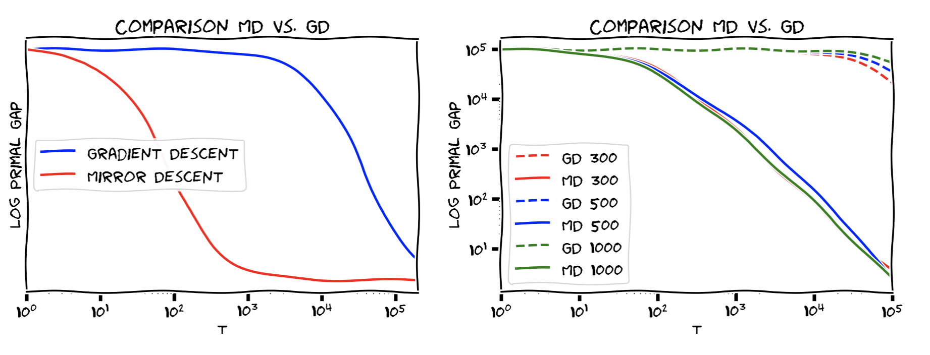
Below we compare Mirror Descent and Gradient Descent over $K = \Delta_n$ with $n = 10000$ (left) and across different values of $n$ on the (right) for some randomly generated functions; both plots are log-log plots. As can be seen Mirror Descent can scale much better than Gradient Descent by choosing a Bregman divergence that is optimized for the geometry. For $K = \Delta_n$, the dependence on $n$ for Mirror Descent (with relative entropy and $\ell_1$-norm) is only logarithmic vs. for Gradient Descent it is linear in the dimension $n$. This logarithmic dependency makes Mirror Descent well suited for large-scale applications in this case.
Extensions
Finally I will talk about some natural extensions. While the full arguments will be beyond the scope, the interested reader might consult [Z2] for proofs. Also, there are various natural extensions in the online learning case, e.g., where we compare to slowly changing strategies; see [Z] for details.
Stochastic versions
It is relatively easy to see that the above bounds can be transferred to the stochastic setting, where we have an unbiased (sub-)gradient estimator only. We then obtain basically the same convergence rates and regret bounds in expectation.
More specifically, see [LNS] for details, for unbiased stochastic subgradients $\partial f(x,\xi)$ ($\xi$ is a random variable), so that their variance is bounded, i.e.,
\[\mathbb E[\norm{\partial f(x,\xi)}_\esx^2] \leq M_\esx^2,\]one can achieve (using Mirror Descent) a guarantee of:
\[\mathbb E \left[f(x_T) - f(x^\esx)\right] \leq O\left(\frac{\sqrt{2} D M_\esx}{\sqrt{\alpha}\sqrt{T}}\right),\]where $D$ is the “diameter” of the feasible region w.r.t. to the distance generating function used in the Bregman divergence. Note that the iterates $x_t$ are random now depending on the realizations of the $\xi$ when sampling (sub-)gradients. Moreover, via Markov’s inequality one can prove probabilistic statements of the form:
\[\mathbb P\left[f(x_T) - f(x^\esx) > \varepsilon \right]\leq O(1) \frac{\sqrt{2} D M_\esx}{\varepsilon \sqrt{\alpha}\sqrt{T}}.\]Smooth case
When $f$ is smooth we can modify (basicMD) to obtain the improved $O(1/t)$ rate. Recall that $f$ is $L$-smooth with respect to $\norm{\cdot}$ if:
\[\tag{smooth} f(y) - f(x) \leq \langle \nabla f(x), y-x \rangle + \frac{L}{2} \norm{x-y}^2.\]for all $x,y \in \mathbb R^n$. Choosing $x \leftarrow x_t$ and $y \leftarrow x_{t+1}$ we obtain:
\[\begin{align*} \langle \nabla f(x_t), x_{t+1} - x^\esx \rangle & = \langle \nabla f(x_t), x_{t} - x^\esx \rangle + \langle \nabla f(x_t), x_{t+1} - x_t \rangle \\ & \geq f(x_t) - f(x^\esx) + f(x_{t+1}) - f(x_t) - \frac{L}{2} \norm{x_{t+1}-x_t}^2 \\ & = f(x_{t+1}) - f(x^\esx) - \frac{L}{2} \norm{x_{t+1}-x_t}^2 \end{align*}\]We now modify (basicMD) with $u = x^\esx$ as follows:
\[\tag{basicMDSmooth} \begin{align*} \langle \eta_t \nabla f(x_t),x_{t+1} - x^\esx \rangle & \leq - \langle \nabla V_{x_t}(x_{t+1}), x_{t+1} - x^\esx \rangle \\ & = V_{x_t}(x^\esx) - V_{x_{t+1}}(x^\esx) - V_{x_t}(x_{t+1}). \end{align*}\]Chaining in the inequality we obtained from smoothness:
\[\begin{align*} \eta_t (f(x_{t+1}) - f(x^\esx)) & \leq \langle \eta_t \nabla f(x_t),x_{t+1} - x^\esx \rangle + \eta_t \frac{L}{2} \norm{x_{t+1}-x_t}^2 \\ & \leq - \langle \nabla V_{x_t}(x_{t+1}), x_{t+1} - x^\esx \rangle + \eta_t \frac{L}{2} \norm{x_{t+1}-x_t}^2 \\ & = V_{x_t}(x^\esx) - V_{x_{t+1}}(x^\esx) - V_{x_t}(x_{t+1}) + \eta_t \frac{L}{2} \norm{x_{t+1}-x_t}^2 \\ & \leq V_{x_t}(x^\esx) - V_{x_{t+1}}(x^\esx) - \frac{1}{2} \norm{x_{t+1}-x_t}^2 + \eta_t \frac{L}{2} \norm{x_{t+1}-x_t}^2, \end{align*}\]where the last inequality used the compatibility of the Bregman divergence with the norm. Picking $\eta_t = \frac{1}{L}$ results in
\[\frac{1}{L} (f(x_{t+1}) - f(x^\esx)) \leq V_{x_t}(x^\esx) - V_{x_{t+1}}(x^\esx),\]which we telescope out to
\[\sum_{t = 0}^{T-1} (f(x_{t+1}) - f(x^\esx)) \leq L V_{x_0}(x^\esx),\]and by convexity the average $\bar x = \frac{1}{T} \sum_{t = 0}^{T-1} x_t$ satisfies:
\[f(\bar x) - f(x^\esx) \leq \frac{L V_{x_0}(x^\esx)}{T},\]which is the expected rate for the smooth case. Note that this improvement does not translate to the online case.
Strongly convex case
Finally we will show that if $f$ is $\mu$-strongly convex with respect to $V_x(y)$ (not necessarily smooth though), then we can also obtain improved rates. This improvement translates also to the online learning case, i.e., we get the corresponding improvement in regret. Recall that a function is $\mu$-strongly convex with respect to $V_x(y)$ if:
\[f(y) - f(x) \geq \langle \nabla f(x),y-x \rangle + \mu V_x(y),\]holds for all $x,y \in \mathbb R^n$. Choosing $x \leftarrow x_t$ and $y \leftarrow x^\esx$, we obtain:
\[\langle \nabla f(x_t), x_t - x^\esx \rangle \geq f(x_t) - f(x^\esx) + \mu V_{x_t}(x^\esx).\]Again we start with (basicMD), which we will modify:
\[\begin{align*} \langle \eta_t \nabla f(x_t),x_{t} - x^\esx \rangle & \leq V_{x_t}(x^\esx) - V_{x_{t+1}}(x^\esx) + \frac{\eta_t^2}{2}\norm{\partial f(x_t)}_\esx^2. \end{align*}\]We now plug in the bound from strong convexity to obtain:
\[\begin{align*} \eta_t (f(x_t) - f(x^\esx) + \mu V_{x_t}(x^\esx)) & \leq \langle \eta_t \nabla f(x_t),x_{t} - x^\esx \rangle \\ & \leq V_{x_t}(x^\esx) - V_{x_{t+1}}(x^\esx) + \frac{\eta_t^2}{2}\norm{\partial f(x_t)}_\esx^2, \end{align*}\]which can be simplified to
\[\tag{basicMDSC} \begin{align*} \eta_t (f(x_t) - f(x^\esx)) & \leq V_{x_t}(x^\esx) - V_{x_{t+1}}(x^\esx) + \frac{\eta_t^2}{2}\norm{\partial f(x_t)}_\esx^2 - \eta_t \mu V_{x_t}(x^\esx) \\ & \leq \left(1- \eta_t \mu\right) V_{x_t}(x^\esx) - V_{x_{t+1}}(x^\esx) + \frac{\eta_t^2}{2}\norm{\partial f(x_t)}_\esx^2. \end{align*}\]Choosing $\eta_t = \frac{1}{\mu t}$ now we obtain:
\[\begin{align*} \frac{1}{\mu t} (f(x_t) - f(x^\esx)) & \leq \left(1- \frac{1}{t}\right) V_{x_t}(x^\esx) - V_{x_{t+1}}(x^\esx) + \frac{1}{2\mu^2t^2}\norm{\partial f(x_t)}_\esx^2 \\ \Leftrightarrow \frac{1}{\mu} (f(x_t) - f(x^\esx)) & \leq \left(t- 1\right) V_{x_t}(x^\esx) - t V_{x_{t+1}}(x^\esx) + \frac{1}{2\mu^2t}\norm{\partial f(x_t)}_\esx^2, \end{align*}\]which we can finally sum up (starting at $t=1$), multiply by $\mu$, and telescope out to arrive at:
\[\begin{align*} \sum_{t = 1}^{T} (f(x_t) - f(x^\esx)) & \leq - T \mu V_{x_{T+1}}(x^\esx) + \frac{G^2}{2\mu} \sum_{t = 1}^{T-1} \frac{1}{t} \leq \frac{G^2 \log T}{2\mu}, \end{align*}\]and with the usual averaging and using convexity we obtain:
\[f(\bar x) - f(x^\esx) \leq \frac{G^2 \log T}{2\mu T}\]for the convergence rate and
\[\sum_{t = 0}^{T-1} f_t(x_t) - \min_x \sum_{t = 0}^{T-1} f_t(x) \leq \frac{G^2 }{2\mu} \log T,\]for the regret; note that this bound is already anytime. In order to obtain the regret bound, simply replace $x^\esx$ by an arbitrary $u$ and $f(x_t)$ by $f_t(x_t)$. Note however, that this time the argument is directly on the primal difference $f_t(x_t) - f_t(u)$, rather than the dual gaps, i.e., after plugging-in the strong convexity inequality we start from:
\[\begin{align*} \eta_t (f_t(x_t) - f_t(u) + \mu V_{x_t}(u)) & \leq \langle \eta_t \nabla f_t(x_t), x_{t} - u \rangle \\ & \leq V_{x_t}(u) - V_{x_{t+1}}(u) + \frac{\eta_t^2}{2}\norm{\partial f_t(x_t)}_\esx^2, \end{align*}\]and continue the same way.
References
[NY] Nemirovsky, A. S., & Yudin, D. B. (1983). Problem complexity and method efficiency in optimization.
[BT] Beck, A., & Teboulle, M. (2003). Mirror descent and nonlinear projected subgradient methods for convex optimization. Operations Research Letters, 31(3), 167-175. pdf
[Z] Zinkevich, M. (2003). Online convex programming and generalized infinitesimal gradient ascent. In Proceedings of the 20th International Conference on Machine Learning (ICML-03) (pp. 928-936). pdf
[AO] Allen-Zhu, Z., & Orecchia, L. (2014). Linear coupling: An ultimate unification of gradient and mirror descent. arXiv preprint arXiv:1407.1537. pdf
[AHK] Arora, S., Hazan, E., & Kale, S. (2012). The multiplicative weights update method: a meta-algorithm and applications. Theory of Computing, 8(1), 121-164. pdf
[Z2] Zhang, X. Bregman Divergence and Mirror Descent. pdf
[LNS] Lan, G., Nemirovski, A., & Shapiro, A. (2012). Validation analysis of mirror descent stochastic approximation method. Mathematical programming, 134(2), 425-458. pdf
[MS] Mcmahan, B., & Streeter, M. (2012). No-regret algorithms for unconstrained online convex optimization. In Advances in neural information processing systems (pp. 2402-2410). pdf
Changelog
03/02/2019: Fixed several typos and added clarifications as pointed out by Matthieu Bloch.
03/04/2019: Fixed several typos and a norm/divergence mismatch in the strongly convex case as pointed out by Cyrille Combettes.
05/15/2019: Added pointer to stochastic case and summary of the results in this case.
08/25/2019: Added brief discussion about no-regret algorithms in the unconstrained online learning setting and a pointer to [MS] as pointed out by Francesco Orabona.
Comments