Cheat Sheet: Smooth Convex Optimization
TL;DR: Cheat Sheet for smooth convex optimization and analysis via an idealized gradient descent algorithm. While technically a continuation of the Frank-Wolfe series, this should have been the very first post and this post will become the Tour d’Horizon for this series. Long and technical.
Posts in this series (so far).
- Cheat Sheet: Smooth Convex Optimization
- Cheat Sheet: Frank-Wolfe and Conditional Gradients
- Cheat Sheet: Linear convergence for Conditional Gradients
- Cheat Sheet: Hölder Error Bounds (HEB) for Conditional Gradients
- Cheat Sheet: Subgradient Descent, Mirror Descent, and Online Learning
- Cheat Sheet: Acceleration from First Principles
My apologies for incomplete references—this should merely serve as an overview.
In this fourth installment of the series on Conditional Gradients, which actually should have been the very first post, I will talk about an idealized gradient descent algorithm for smooth convex optimization, which allows to obtain convergence rates and from which we can instantiate several known algorithms, including gradient descent and Frank-Wolfe variants. This post will become a Tour d’Horizon of the various results from this series. To be clear, the focus is on projection-free methods in the constraint case, however I will deal with other approaches to complement the exposition.
While I will use notation that is compatible with previous posts, in particular the first post, I will make this post as self-contained as possible with few forward references, so that this will become “Post Zero”. As before I will use Frank-Wolfe [FW] and Conditional Gradients [CG] interchangeably.
Our setup will be as follows. We will consider a convex function $f: \RR^n \rightarrow \RR$ and we want to solve
\[\min_{x \in K} f(x),\]where $K$ is some feasible region, e.g., $K = \RR^n$ is the unconstrained case. We will in particular consider smooth functions as detailed further below and we assume that we only have first-order access to the function, via a so-called first-order oracle:
First-Order oracle for $f$
Input: $x \in \mathbb R^n$
Output: $\nabla f(x)$ and $f(x)$
For now we disregard how we can access the feasible region $K$ as there are various access models and we will specify the model based on the algorithmic class that we target later. For the sake of simplicity, we will be using the $\ell_2$-norm but the arguments can be easily extended to other norms, e.g., replacing Cauchy-Schwartz inequalities by Hölder inequalities and using dual norms.
An idealized gradient descent algorithm
In a first step we will devise an idealized gradient descent algorithm, for which we will then derive convergence guarantees under different assumptions on the function $f$ under consideration. We will then show how known guarantees can be easily obtained from this idealized gradient descent algorithm.
Let $f: \RR^n \rightarrow \RR$ be a convex function and $K$ be some feasible region. We are interested in studying ‘gradient descent-like’ algorithms. To this end let $x_t \in K$ be some point and we consider updates of the form
\[ \tag{dirStep} x_{t+1} \leftarrow x_t - \eta_t d_t, \]
for some direction $d_t \in \RR^n$ and $\eta_t \in \RR$ for $t$. For example, we would obtain standard gradient descent by choosing $d \doteq \nabla f(x_t)$ and $\eta_t = \frac{1}{L}$, where $L$ is the Lipschitz constant of $f$.
Measures of progress
We will consider two important measures that drive the overall convergence rate. The first is a measure of progress, which in our context will be provided by the smoothness of the function. This will be the only measure of progress that we will consider, but there are many others for different setups. Note that the arguments here using smoothness do not rely on the convexity of the function; something to remember for later.
Let us recall the definition of smoothness:
Definition (smoothness). A convex function $f$ is said to be $L$-smooth if for all $x,y \in \mathbb R^n$ it holds: \[ f(y) - f(x) \leq \langle \nabla f(x), y-x \rangle + \frac{L}{2} \norm{x-y}^2. \]
There are two things to remember about smoothness:
- If $x$ is an optimal solution to (the unconstrained) $f$, then $\nabla f(x) = 0$, so that smoothness provides an upper bound on the distance to optimality: $f(x) - f(x^\esx) \leq \frac{L}{2} \norm{x-x^\esx}^2$.
- More generally it provides an upper bound for the change of the function by means of a quadratic.
The most important thing however is that smoothness induces progress in schemes such as (dirStep). For this let us consider the smoothness inequality at two iterates $x_t$ and $x_{t+1}$ in the scheme from above. Plugging in the definition of (dirStep) we obtain
\[\underbrace{f(x_{t}) - f(x_{t+1})}_{\text{primal progress}} \geq \eta \langle\nabla f(x_t),d\rangle - \eta^2 \frac{L}{2} \|d\|^2\]Note that the function on the right is concave in $\eta$ and so we can maximize the right-hand side to obtain a lower bound on the progress. Taking the derivative on the right-hand side and asserting criticality we obtain:
\[\langle\nabla f(x_t),d\rangle - \eta L \norm{d}^2 = 0,\]which leads to the optimal choice $\eta^\esx \doteq \frac{\langle\nabla f(x_t),d\rangle}{L \norm{d}^2}$. This induces a progress lower bound of:
Progress induced by smoothness (for $d$). \[ \begin{equation} \tag{Progress from $d$} \underbrace{f(x_{t}) - f(x_{t+1})}_{\text{primal progress}} \geq \frac{\langle\nabla f(x_t),d\rangle^2}{2L \norm{d}^2}. \end{equation} \]
We will now formulate our idealized gradient descent by using the (normalized) idealized direction $d \doteq \frac{x_t - x^\esx}{\norm{ x_t - x^\esx }}$, where we basically make steps in the direction of the optimal solution $x^\esx$; note that in general there might be multiple optimal solutions, in which case we choose arbitrarily but fixed.
Idealized Gradient Descent (IGD)
Input: Smooth convex function $f$ with first-order oracle access and smoothness parameter $L$.
Output: Sequence of points $x_0, \dots, x_T$
For $t = 0, \dots, T-1$ do:
$\quad x_{t+1} \leftarrow x_t - \eta_t \frac{x_t - x^\esx}{\norm{ x_t - x^\esx }}$ with $\eta_t = \frac{\langle\nabla f(x_t),\frac{x_t - x^\esx}{\norm{ x_t - x^\esx }}\rangle}{L}$
It is important to note that in reality we do not have access to this idealized direction. Moreover, if we would have access, we could perform line search along this direction to get the optimal solution $x^\esx$ in a single step. However, what we assume here is that the algorithm does not know that this is an optimal direction and hence only having first-order access, the smoothness condition, and assuming that we do not do line search etc., the best the algorithm can do is use the optimal step length from smoothness, which is exactly how we choose $\eta_t$. Also note, that we could have defined $d$ as the unnormalized idealized direction $x_t - x^\esx$, however the normalization simplifies exposition.
Let us now briefly establish the progress guarantees for IGD. For the sake of brevity let $h_t \doteq h(x_t) \doteq f(x_t) - f(x^\esx)$ denote the primal gap (at $x_t$). Plugging in the parameters into the progress inequality, we obtain
Progress guarantee for IGD. \[ \begin{equation} \tag{IGD Progress} \underbrace{f(x_{t}) - f(x_{t+1})}_{\text{primal progress}} = h_{t} - h_{t+1} \geq \frac{\langle \nabla f(x_t),x_t - x^\esx \rangle^2}{2L \norm{x_t - x^\esx}^2}. \end{equation} \]
Measures of optimality
We will now introduce measures of optimality that together with (IGD Progress) induce convergence rates for IGD. These rates are idealized rates as they depend on the idealized direction, nonetheless we will see that actual rates for known algorithms almost immediately follow from here in the following section. We will start with some basic measures first; I might expand this list over time if I come across other measures that can be explained relatively easily.
In order to establish (idealized) convergence rates, we have to relate $\langle \nabla f(x_t),x_t - x^\esx \rangle$ with $f(x_t) - f(x^\esx)$. There are many different such relations that we refer to as measures of optimality, as they effectively provide a guarantee on the primal gap $h_t$ via dual information as will become clear soon.
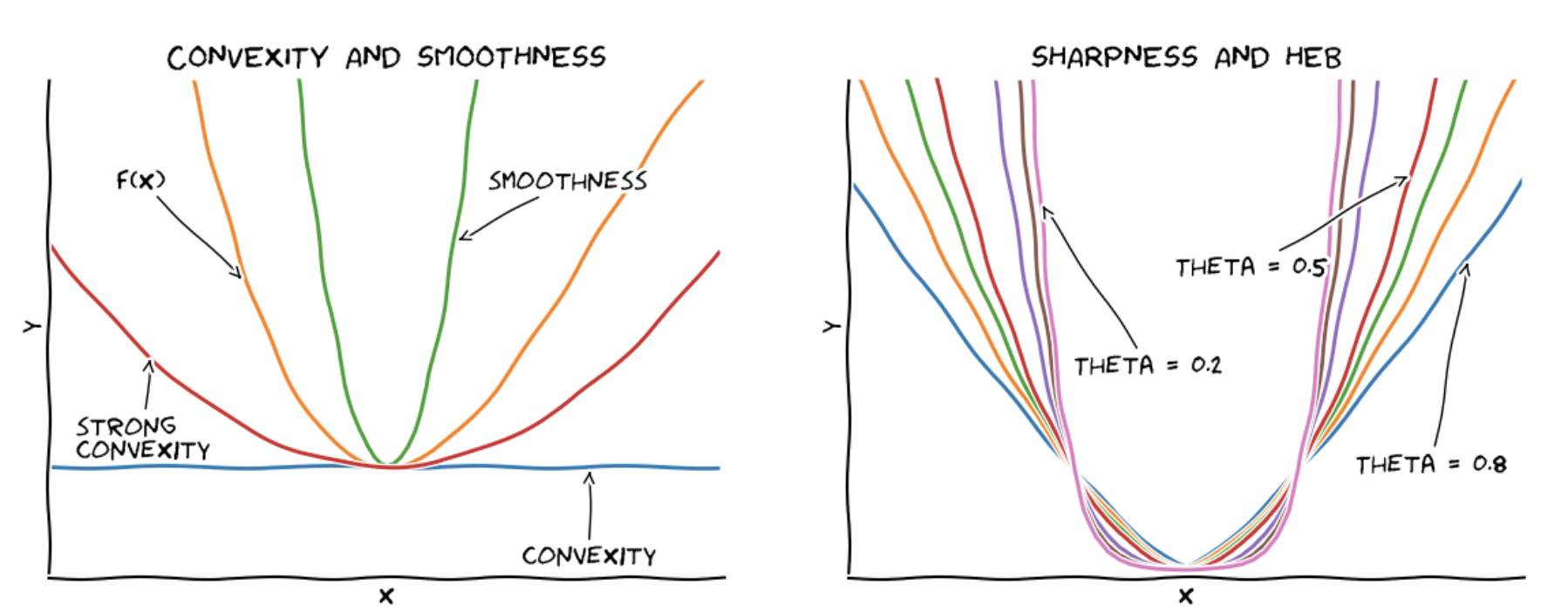
To put things into perspective, smoothness provides a quadratic upper bound on $f(x)$, while convexity provides a linear lower bound on $f(x)$ and strong convexity provides a quadratic lower bound on $f(x)$. The HEB condition (to be introduced later), which will be one of the considered measures of optimality, basically interpolates between linear and quadratic lower bounds by capturing how sharp the function curves around the optimal solution(s). The following graphics shows the relation between convexity, strong convexity, and smoothness on the left and functions with different $\theta$-values in the HEB condition (as explained further below) on the right.
Convexity
Our first measure of optimality is convexity.
Definition (convexity). A differentiable function $f$ is said to be convex if for all $x,y \in \mathbb R^n$ it holds: \[f(y) - f(x) \geq \langle \nabla f(x), y-x \rangle.\]
From this we can derive a very basic guarantee on the primal gap $h_t$, by choosing $y \leftarrow x^\esx$ and $x \leftarrow x_t$ and we obtain:
Primal Bound (convexity). At an iterate $x_t$ convexity induces a primal bound of the form: \[ \tag{PB-C} f(x_t) - f(x^\esx) \leq \langle \nabla f(x_t),x_t - x^\esx \rangle. \]
Combining (PB-C) with (IGD-Progress) we obtain:
\[h_{t} - h_{t+1} \geq \frac{\langle \nabla f(x_t),x_t - x^\esx \rangle^2}{2L \norm{x_t - x^\esx}^2} \geq \frac{h_t^2}{2L \norm{x_t - x^\esx}^2} \geq \frac{h_t^2}{2L \norm{x_0 - x^\esx}^2},\]where the last inequality is not immediate but also not hard to show. Rearranging things we obtain:
IGD contraction (convexity). Assuming convexity the primal gap $h_t$ contracts as: \[ \tag{Rec-C} h_{t+1} \leq h_t \left(1 - \frac{h_t}{2L \norm{x_0 - x^\esx}^2}\right), \] which leads to a convergence rate after solving the recurrence of \[ \tag{Rate-C} h_T \leq \frac{2L \norm{x_0 - x^\esx}^2}{T+4}. \]
Strong Convexity
Our second measure of optimality is strong convexity.
Definition (strong convexity). A convex function $f$ is said to be $\mu$-strongly convex if for all $x,y \in \mathbb R^n$ it holds: \[ f(y) - f(x) \geq \langle \nabla f(x),y-x \rangle + \frac{\mu}{2} \norm{x-y}^2. \]
The strong convexity inequality is basically the reverse inequality of smoothness and we can use an argument similar to the one we used for the progress bound. For this we choose $x \leftarrow x_t$ and $y \leftarrow x_t - \eta e_t$ with $e_t \doteq x_t - x^\esx = d_t \norm{x_t-x^\esx}$ being the unnormalized idealized direction to obtain:
\[f(x_t - \eta e_t) - f(x_t) \geq - \eta \langle\nabla f(x_t),e_t\rangle + \eta^2\frac{\mu}{2} \| e_t \|^2.\]Now we minimize the right-hand side over $\eta$ and obtain that the minimum is achieved for the choice $\eta^\esx \doteq \frac{\langle\nabla f(x_t), e_t\rangle}{\mu \norm{e_t}^2}$; this is basically the same form as the $\eta^*$ from above. Plugging this back in, we obtain
\[f(x_t) - f(x_t - \eta e_t) \leq \frac{\langle\nabla f(x_t),e_t\rangle^2}{2 \mu \norm{e_t}^2},\]and as the right-hand side is now independent of $\eta$, we can in particular choose $\eta = 1$ and obtain:
Primal Bound (strong convexity). At an iterate $x_t$ strong convexity induces a primal bound of the form: \[ \tag{PB-SC} f(x_t) - f(x^\esx) \leq \frac{\langle \nabla f(x_t),x_t - x^\esx \rangle^2}{2\mu \norm{x_t - x^\esx}^2}. \]
Combining (PB-SC) with (IGD-Progress) we obtain:
\[h_{t} - h_{t+1} \geq \frac{\langle \nabla f(x_t),x_t - x^\esx \rangle^2}{2L \norm{x_t - x^\esx}^2} \geq \frac{\mu}{L} h_t.\]IGD contraction (strong convexity). Assuming strong convexity the primal gap $h_t$ contracts as: \[ \tag{Rec-SC} h_{t+1} \leq h_t \left(1 - \frac{\mu}{L}\right), \] which leads to a convergence rate after solving the recurrence of \[ \tag{Rate-SC} h_T \leq \left(1 - \frac{\mu}{L}\right)^T h_0 \leq e^{-\frac{\mu}{L}T}h_0. \] or equivalently, $h_T \leq \varepsilon$ for \[ T \geq \frac{L}{\mu} \log \frac{h_0}{\varepsilon}. \]
Hölder Error Bound (HEB) Condition
One might wonder whether there are rates between those induced by convexity and those induced by strong convexity. This brings us to the Hölder Error Bound (HEB) condition that interpolates smoothly between the two regimes. Here we will confine the discussion to the basics that induce the bounds that we need; for an in-depth discussion and relation to e.g., the dominated gradient property, see the HEB post in this series. Let $K^\esx$ denote the set of optimal solutions to $\min_{x \in K} f(x)$ and let $f^\esx \doteq f(x)$ for some $x \in K^\esx$.
Definition (Hölder Error Bound (HEB) condition). A convex function $f$ is satisfies the Hölder Error Bound (HEB) condition on $K$ with parameters $0 < c < \infty$ and $\theta \in [0,1]$ if for all $x \in K$ it holds: \[ c (f(x) - f^\esx)^\theta \geq \min_{y \in K^\esx} \norm{x-y}. \]
Note that in contrast to convexity and strong convexity the HEB condition is a local condition as can be seen from its definition. As we assume that our functions are smooth it follows $\theta \leq 1/2$ (see HEB post for details). We can now combine (HEB) for any $x^\esx \in K^\esx$ with convexity to obtain:
\[\begin{align*} f(x) - f^\esx & = f(x) - f(x^\esx) \leq \langle \nabla f(x), x - x^\esx \rangle \\ & = \frac{\langle \nabla f(x), x - x^\esx \rangle}{\norm{x - x^\esx}} \norm{x - x^\esx} \\ & \leq \frac{\langle \nabla f(x), x - x^\esx \rangle}{\norm{x - x^\esx}} c (f(x) - f^\esx)^\theta. \end{align*}\]Via rearranging we derive: \[ \frac{1}{c}(f(x) - f^\esx)^{1-\theta} \leq \frac{\langle \nabla f(x), x - x^\esx \rangle}{\norm{x - x^\esx}}. \]
Primal Bound (HEB). At an iterate $x_t$ HEB induces a primal bound of the form: \[ \tag{PB-HEB} \frac{1}{c}(f(x_t) - f^\esx)^{1-\theta} \leq \frac{\langle \nabla f(x_t), x_t - x^\esx \rangle}{\norm{x_t - x^\esx}} \] for any $x^\esx \in K^\esx$.
Combining (PB-HEB) with (IGD-Progress) we obtain:
\[h_t - h_{t+1} \geq \frac{\langle \nabla f(x_t), x_t - x^\esx\rangle^2}{2L \norm{x_t - x^\esx}^2} \geq \frac{\left(\frac{1}{c}h_t^{1-\theta} \right)^2}{2L},\]which can be rearranged to:
\[h_{t+1} \leq h_t - \frac{\frac{1}{c^2}h_t^{2-2\theta}}{2L} \leq h_t \left(1 - \frac{1}{2Lc^2} h_t^{1-2\theta}\right).\]IGD contraction (HEB). Assuming HEB the primal gap $h_t$ contracts as: \[ \tag{Rec-HEB} h_{t+1} \leq h_t \left(1 - \frac{1}{2Lc^2} h_t^{1-2\theta}\right), \] which leads to a convergence rate after solving the recurrence of \[ \tag{Rate-HEB} h_T \leq \begin{cases} \left(1 - \frac{1}{2Lc^2}\right)^T h_0 & \theta = 1/2 \newline O(1) \left(\frac{1}{T} \right)^\frac{1}{1-2\theta} & \text{if } \theta < 1/2 \end{cases} \] or equivalently for the latter case, to ensure $h_T \leq \varepsilon$ it suffices to choose $T \geq \Omega\left(\frac{1}{\varepsilon^{1 - 2\theta}}\right)$. Note that the $O(1)$ term hides the dependence on $h_0$ for simplicity of exposition.
Obtaining known algorithms
We will now derive several known algorithms and results using IGD from above. The basic task that we have to accomplish is always the same. We show that the direction $d_t$ that our algorithm under consideration takes in iteration $t$ satisfies:
\[ \tag{Scaling} \frac{\langle \nabla f(x_t),d_t \rangle}{\norm{d_t}} \geq \alpha_t \frac{\langle \nabla f(x_t), x_t - x^\esx \rangle}{\norm{x_t - x^\esx}}, \]
for some $\alpha_t \geq 0$. The reason why we want to show (Scaling) is that, assuming that we use the optimal step length $\eta_t^\esx = \frac{\langle\nabla f(x_t),d_t\rangle}{L \norm{d_t}^2}$ from the smoothness equation, this ensures that for the progress from our step it holds:
\[ \tag{ProgressApprox} h_t - h_{t+1} \geq \frac{\langle \nabla f(x_t),d_t \rangle^2}{2L\norm{d_t}^2} \geq \alpha_t^2 \frac{\langle \nabla f(x_t),x_t - x^\esx \rangle^2}{2L\norm{x_t - x^\esx}^2}, \]
so that we lose the approximation factor $\alpha_t^2$ in the primal progress inequality. Usually, we will see that we can compute a constant $\alpha_t = \alpha > 0$ for all $t$. This allows us to immediately apply all previous convergence bounds derived for IGD, corrected by the approximation factor $\alpha^2$ that we (might) lose now in each iteration.
Note, that for several of the algorithms presented below accelerated variants can be obtained, so that the presented rates are not optimal; I will address this and talk about acceleration in a future post. In general the method via IGD might not necessarily provide the sharpest constants etc but rather favors simplicity of exposition.
Gradient Descent
We will start with the (vanilla) Gradient Descent (GD) algorithms in the unconstrained setting, i.e., $K = \RR^n$.
(Vanilla) Gradient Descent (GD)
Input: Smooth convex function $f$ with first-order oracle access, initial point $x_0 \in \RR^n$.
Output: Sequence of points $x_0, \dots, x_T$
For $t = 0, \dots, T-1$ do:
$\quad x_{t+1} \leftarrow x_t - \gamma_t \nabla f(x_t)$
In order to show (Scaling) for $d_t \doteq \nabla f(x_t)$ consider: \[ \tag{ScalingGD} \frac{\langle \nabla f(x_t),\nabla f(x_t) \rangle}{\norm{\nabla f(x_t)}} = \norm{\nabla f(x_t)} \geq \frac{\langle \nabla f(x_t), x_t - x^\esx \rangle}{\norm{x_t - x^\esx}}, \] by Cauchy-Schwarz, so that we can choose $\alpha_t = 1$ for all $t \in [T]$. In order to obtain (ProgressApprox) we pick the optimal step length $\gamma_t^\esx = \frac{\langle\nabla f(x_t),d_t\rangle}{L \norm{d_t}^2} = \frac{1}{L}$.
We now obtain the convergence rate by simply combining the approximation from above with the IGD convergence rates. These bounds readily follow from plugging-in and we only copy-and-paste them here for completeness.
General convergence for smooth functions
For the (general) smooth case we obtain:
GD contraction (convexity). Assuming convexity the primal gap $h_t$ contracts as: \[ \tag{GD-Rec-C} h_{t+1} \leq h_t \left(1 - \frac{h_t}{2L \norm{x_0 - x^\esx}^2}\right), \] which leads to a convergence rate after solving the recurrence of \[ \tag{GD-Rate-C} h_T \leq \frac{2L \norm{x_0 - x^\esx}^2}{T+4}. \]
Linear convergence for strongly convex functions
For smooth and strongly convex functions we obtain:
GD contraction (strong convexity). Assuming strong convexity the primal gap $h_t$ contracts as: \[ \tag{GD-Rec-SC} h_{t+1} \leq h_t \left(1 - \frac{\mu}{L}\right), \] which leads to a convergence rate after solving the recurrence of \[ \tag{GD-Rate-SC} h_T \leq \left(1 - \frac{\mu}{L}\right)^T h_0 \leq e^{-\frac{\mu}{L}T}h_0. \] or equivalently, $h_T \leq \varepsilon$ for \[ T \geq \frac{L}{\mu} \log \frac{h_0}{\varepsilon}. \]
HEB rates
And for smooth functions satisfying the HEB condition we obtain:
GD contraction (HEB). Assuming HEB the primal gap $h_t$ contracts as: \[ \tag{GD-Rec-HEB} h_{t+1} \leq h_t \left(1 - \frac{1}{2Lc^2} h_t^{1-2\theta}\right), \] which leads to a convergence rate after solving the recurrence of \[ \tag{GD-Rate-HEB} h_T \leq \begin{cases} \left(1 - \frac{1}{2Lc^2}\right)^T h_0 & \theta = 1/2 \newline O(1) \left(\frac{1}{T} \right)^\frac{1}{1-2\theta} & \text{if } \theta < 1/2 \end{cases} \] or equivalently for the latter case, to ensure $h_T \leq \varepsilon$ it suffices to choose $T \geq \Omega\left(\frac{1}{\varepsilon^{1 - 2\theta}}\right)$. Note that the $O(1)$ term hides the dependence on $h_0$ for the simplicity of exposition.
Projected Gradient Descent
The route through IGD is flexible enough to also accommodate the constraint case. Now we have to project back into the feasible region $K$ and Projected Gradient Descent (PGD), employs a projection $\Pi_K$ that projects a point $x \in \RR^n$ back into the feasible region $K$ (note that $\Pi_K$ has to satisfy certain properties to be admissible):
Projected Gradient Descent (PGD)
Input: Smooth convex function $f$ with first-order oracle access, initial point $x_0 \in K$.
Output: Sequence of points $x_0, \dots, x_T$
For $t = 0, \dots, T-1$ do:
$\quad x_{t+1} \leftarrow \Pi_K(x_t - \gamma_t \nabla f(x_t))$
Without going into details we obtain (Scaling) here in a similar way due to the properties of the projection; I might explicitly consider projection-based methods in a later post.
Frank-Wolfe Variants
We will now discuss how Frank-Wolfe Variants fit into the IGD framework laid out above. For this, in addition to the first-order access to the function $f$ we now need to specify access to the feasible region $K$, which will be through a linear programming oracle:
Linear Programming oracle
Input: $c \in \mathbb R^n$
Output: $\arg\min_{x \in K} \langle c, x \rangle$
With this we can formulate the (vanilla) Frank-Wolfe algorithm:
Frank-Wolfe Algorithm [FW]
Input: Smooth convex function $f$ with first-order oracle access, feasible region $K$ with linear optimization oracle access, initial point (usually a vertex) $x_0 \in K$.
Output: Sequence of points $x_0, \dots, x_T$
For $t = 0, \dots, T-1$ do:
$\quad v_t \leftarrow \arg\min_{x \in K} \langle \nabla f(x_{t}), x \rangle$
$\quad x_{t+1} \leftarrow (1-\eta_t) x_t + \eta_t v_t$
The Frank-Wolfe algorithm [FW] (also known as Conditional Gradients [CG]) has many advantages with its projection-freeness being one of the most important; see Cheat Sheet: Frank-Wolfe and Conditional Gradients for an in-depth discussion.
Before, we continue we need to address a small technicality: In the argumentation so far we did not have any restriction on choosing the step length $\eta$. However, in the case of Frank-Wolfe, as we are forming convex combinations, we have $0\leq \eta \leq 1$ to ensure feasibility. Formally, we would have to distinguish two cases, namely, where $\eta^\esx = \frac{\langle \nabla f(x_t), x_t - v_t\rangle}{L \norm{x_t - v_t}^2} \geq 1$ and $\eta^\esx < 1$; note that we always have nonnegativity as $\langle \nabla f(x_t), x_t - v_t\rangle \geq 0$. We will purposefully disregard the former case, because in this regime we have linear convergence (the best we can hope for) anyways and as such it is really the iterations with $\eta < 1$, which determine the convergence rate. Before we continue, we briefly provide a proof of linear convergence when $\eta \geq 1$ in which case we simply choose $\eta \doteq 1$ so that $x_{t+1} = v_t$; moreover we will also establish that this case typically only happens once. By smoothness and using that in this case it holds $\langle \nabla f(x_t), x_t - v_t\rangle \geq L \norm{x_t - v_t}^2$ we have:
\[\tag{LongStep} \begin{align*} \underbrace{f(x_{t}) - f(x_{t+1})}_{\text{primal progress}} & \geq \langle\nabla f(x_t),x_t - v_t\rangle - \frac{L}{2} \norm{x_t - v_t}^2 \newline & \geq \frac{1}{2} \langle\nabla f(x_t),x_t - v_t\rangle \newline & \geq \frac{1}{2} h_t, \end{align*}\]so that in this regime we contract as
\[h_{t+1} \leq \frac{1}{2} h_t\]This can happen only a logarithmic number of steps until $\eta^\esx < 1$ has to hold. Moreover, after one step it is guaranteed that $h_1 \leq \frac{LD^2}{2}$: We start from (LongStep), however we estimate differently; in the following and further below let $D$ denote the diameter of $K$ with respect to $\norm{\cdot}$:
\[\begin{align*} \underbrace{f(x_{0}) - f(x_{1})}_{\text{primal progress}} & \geq \langle\nabla f(x_0),x_0 - v_0\rangle - \frac{L}{2} \norm{x_0 - v_0}^2 \newline & \geq h_0 - \frac{LD^2}{2}. \end{align*}\]Therefore we have for $h_1$:
\[h_1 \leq h_0 - \left(h_0 - \frac{LD^2}{2}\right) \leq \frac{LD^2}{2}.\]Convergence for Smooth Convex Functions
We will now first establish the convergence rate in the (general) smooth case. For this it suffices to observe that:
\[\langle\nabla f(x_t),x_t - v_t\rangle \geq \langle\nabla f(x_t),x_t - x^\esx\rangle \geq 0,\]as $v_t = \arg\min_{x \in K} \langle \nabla f(x_{t}), x \rangle$ and we can rearrange this to:
\[\tag{ScalingFW} \frac{\langle\nabla f(x_t),x_t - v_t\rangle}{\norm{x_t - v_t}} \geq \frac{\norm{x_t - x^\esx}}{D} \cdot \frac{\langle\nabla f(x_t),x_t - x^\esx\rangle}{\norm{x_t - x^\esx}} \geq 0,\]so that the progress per iteration, with $\alpha_t = \frac{\norm{x_t - x^\esx}}{D}$, can be lower bounded by:
\[\tag{ProgressApproxFW} \begin{align*} h_t - h_{t+1} & \geq \frac{\langle \nabla f(x_t),x_t - v_t \rangle^2}{2L\norm{x_t - v_t}^2} \\ & \geq \alpha_t^2 \frac{\langle \nabla f(x_t),x_t - x^\esx \rangle^2}{2L\norm{x_t - x^\esx}^2} \\ & \geq \frac{\langle \nabla f(x_t),x_t - x^\esx \rangle^2}{2LD^2}. \end{align*}\]We obtain for the (general) smooth case:
FW contraction (convexity). Assuming convexity the primal gap $h_t$ contracts as: \[ \tag{FW-Rec-C} h_{t+1} \leq h_t \left(1 - \frac{h_t}{2L D^2}\right), \] which leads to a convergence rate after solving the recurrence of \[ \tag{FW-Rate-C} h_T \leq \frac{2L D^2}{T+4}. \]
Linear convergence for $x^\esx$ in relative interior
Next, we will demonstrate that in the case where $x^\esx$ lies in the relative interior of $K$, then already the vanilla Frank-Wolfe algorithm achieves linear convergence when $f$ is strongly convex. For this we use the following lemma proven in [GM]:
Lemma [GM]. If $x^\esx$ is contained $2r$-deep in the relative interior of $K$, i.e., $B(x^\esx,2r) \cap \operatorname{aff}(K) \subseteq K$ for some $r > 0$, then there exists some $t’$ so that for all $t\geq t’$ it holds \[ \frac{\langle \nabla f(x_t),x_t - v_t\rangle}{\norm{x_t - v_t}} \geq \frac{r}{D} \norm{\nabla f(x_t)}, \] where $v_t = \arg\min_{x \in K} \langle \nabla f(x_{t}), x \rangle$ as above.
In the above $t’$ is the iteration from where onwards it holds $\norm{x_t - x^\esx} \leq r$ for all $t \geq t’$. The lemma establishes (Scaling) with $\alpha_t \doteq \frac{r}{D}$:
\[\tag{ScalingFWint} \frac{\langle \nabla f(x_t),x_t - v\rangle}{\norm{x_t - v}} \geq \frac{r}{D} \norm{\nabla f(x_t)} \geq \frac{r}{D} \frac{\langle\nabla f(x_t),x_t - x^\esx\rangle}{\norm{x_t - x^\esx}}.\]Plugging this into the formula for strongly convex functions and ignoring the initial burn-in phase until we reach $t’$ we obtain:
FW contraction (strong convexity and $x^\esx$ in rel.int). Assuming strong convexity of $f$ and $x^\esx$ being in the relative interior of $K$ with depth $2r$, the primal gap $h_t$ contracts as: \[ \tag{Rec-SC-Int} h_{t+1} \leq h_t \left(1 - \frac{r^2}{D^2} \frac{\mu}{L}\right), \] which leads to a convergence rate after solving the recurrence of \[ \tag{Rate-SC-Int} h_T \leq \left(1 - \frac{r^2}{D^2} \frac{\mu}{L}\right)^T h_0 \leq e^{-\frac{r^2}{D^2} \frac{\mu}{L}T}h_0. \] or equivalently, $h_T \leq \varepsilon$ for \[ T \geq \frac{D^2}{r^2} \frac{L}{\mu} \log \frac{h_0}{\varepsilon}. \]
Note, that it is fine to ignore the burn-in phase before we reach $t’$ as for a function family with optima $x^\esx$ being $2r$-deep in the relative interior of $K$, smoothness parameter $L$, and strong convexity parameter $\mu$, using $\nabla f(x^\esx) = 0$ and strong convexity, in order to satisfy $\norm{x_t - x^\esx} \leq r$ we need $\norm{x_t-x^\esx}^2 \leq \frac{2}{\mu} h_t \leq r^2$ and hence we need to ensure $h_t \leq \frac{\mu}{2} r^2$, which is satisfied after at most $O(\frac{4 LD^2}{\mu r^2})$ iterations, which is a constant for any family satisfying those parameters, so that the asymptotic rate from above is achieved.
The result from above is the best we can hope for using the vanilla Frank-Wolfe algorithm. In particular, if $x^\esx$ is on the boundary linear convergence for strongly convex functions cannot be achieved in general with the vanilla Frank-Wolfe algorithm. Rather it requires a modification of the Frank-Wolfe algorithm that we will discuss further below. For more details, and in particular the lower bound for the case with $x^\esx$ being on the boundary, see Cheat Sheet: Linear convergence for Conditional Gradients.
Improved convergence for strongly convex feasible regions
We will now show that if the feasible region $K$ is strongly convex and the function $f$ is strongly convex, then we can also improve over the standard $O(1/t)$ convergence rate of conditional gradients however it is not known whether we can achieve linear convergence in that case (to the best of my knowledge). Note that we make no assumption here about the location of $x^\esx$. The original result is due to [GH] however the exposition will be different to fit into our IGD framework.
Before we continue, we need to briefly recall strong convexity of a set:
Definition (Strongly convex set). A convex set $K$ is $\alpha$-strongly convex with respect to $\norm{\cdot}$ if for any $x,y \in K$, $\gamma \in [0,1]$, and $z \in \RR^n$ with $\norm{z} = 1$ it holds: \[ \gamma x + (1-\gamma) y + \gamma(1-\gamma)\frac{\alpha}{2}\norm{x-y}^2z \in K. \]
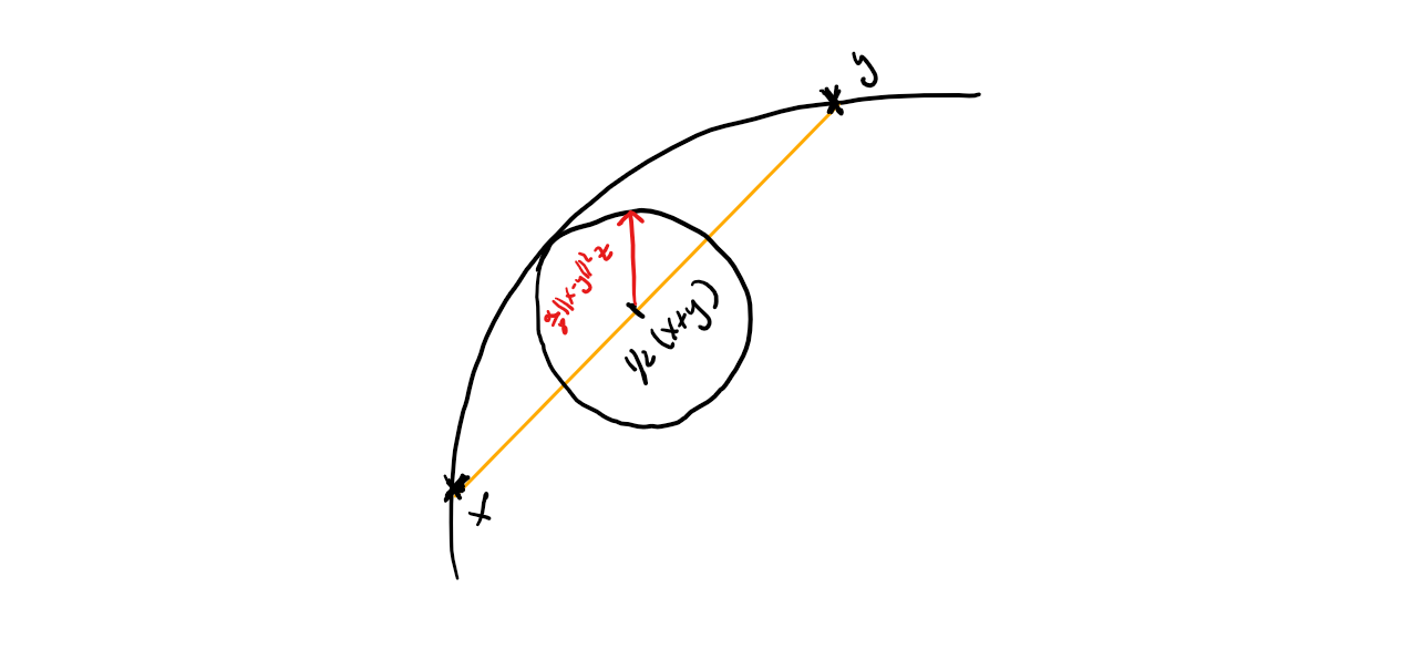
So what this really means is that if you take the line segment between two points then on for any point on that line segment you can squeeze a ball around that point into $K$, where the radius depends on where you are on the line. We will apply the above definition to the mid point of $x$ and $y$, so that the definition ensures that for any $x,y \in K$
\[\tag{SCmidpoint} \frac{1}{2} (x + y) + \frac{\alpha}{8}\norm{x-y}^2z \in K,\]where $z$ is a norm-$1$ direction, as shown in the following graphic:
With this we can easily establish the following variant of (Scaling):
Lemma (Scaling for Strongly Convex Body (SCB)). Let $K$ be a strongly convex set with parameter $\alpha$. Then it holds: \[ \tag{ScalingSCB} \frac{\langle \nabla f(x_t), x_t - v_t \rangle}{\norm{x_t - v_t}^2} \geq \frac{\alpha}{4} \norm{\nabla f(x_t)}, \] where $v_t$ is the Frank-Wolfe point from the algorithm.
Proof. Let $m \doteq \frac{1}{2} (x_t + v_t) + \frac{\alpha}{8}\norm{x_t-v_t}^2 w$, where $w = \arg\min_{w \in \RR^n, \norm{w} = 1} \langle \nabla f(x_t), w \rangle$. Note that $\langle \nabla f(x_t), w \rangle = - \norm{\nabla f(x_t)}$. Now we have:
\[\begin{align*} \langle \nabla f(x_t), x_t - v_t \rangle & \geq \langle \nabla f(x_t), x_t - m \rangle \\ & = \frac{1}{2} \langle \nabla f(x_t), x_t - v_t \rangle - \frac{\alpha}{8} \norm{x_t - v_t}^2 \langle \nabla f(x_t), w \rangle \\ & = \frac{1}{2} \langle \nabla f(x_t), x_t - v_t \rangle + \frac{\alpha}{8} \norm{x_t - v_t}^2 \norm{\nabla f(x_t)}, \end{align*}\]where the first inequality follows from the optimality of the Frank-Wolfe point. From this the statement follows by simply rearranging. $\qed$
This lemma is very much in spirit of the proof of [GM] for $x^\esx$ being in the relative interior of $K$. However, the bound of [GM] is stronger: (ScalingSCB) is not exactly what we need, as we are missing a square around the scalar product in the numerator. This seems to be subtle but it is actually the reason why we do not obtain linear convergence by straightforward plugging-in. In fact, we have to conclude the convergence rate in this case slightly differently by “mixing” the bound from (standard) convexity and (ScalingSCB). Observe that so far, we have not used strong convexity of $f$ yet. Our starting point is the progress inequality from smoothness for the Frank-Wolfe direction $d = x_t - v_t$ and we continue as follows:
\[\begin{align*} f(x_t) - f(x_{t+1}) & \geq \frac{\langle \nabla f(x_t), x_t - v_t \rangle^2}{2L \norm{x_t - v_t}^2} \\ & \geq \langle \nabla f(x_t), x_t - v_t \rangle \cdot \frac{\langle \nabla f(x_t), x_t - v_t \rangle}{2L \norm{x_t - v_t}^2} \\ & \geq h_t \cdot \frac{\alpha}{8L} \norm{\nabla f(x_t)}. \end{align*}\]This leads to a contraction of the form:
\[\tag{Rec-SCB-C} h_{t+1} \leq h_t (1- \frac{\alpha}{8L}\norm{\nabla f(x_t)}),\]and together with strong convexity that ensures
\[h_t \leq \frac{\norm{\nabla f(x_t)}^2}{2\mu}\]we get:
FW contraction (strong convexity and strongly convex body). Assuming strong convexity of $f$ and $K$ is a strongly convex set with parameter $\alpha$, the primal gap $h_t$ contracts as: \[ \tag{Rec-SC-SCB} h_{t+1} \leq h_t \left(1 - \frac{\alpha}{8L}\sqrt{2\mu h_t}\right), \] which leads to a convergence rate after solving the recurrence of \[ \tag{Rate-SC-SCB} h_T \leq O\left(1/T^2\right), \] where the $O(.)$ term hides the dependency on the parameters $L$, $\mu$, and $\alpha$.
Linear convergence for $\norm{\nabla f(x)} > c$
As mentioned above (Rec-SCB-C) does not make any assumptions regarding the strong convexity of the function and in fact we can use this contraction to obtain linear convergence over strongly convex bodies, whenever the lower-bounded gradient assumption holds, i.e., for all $x \in K$, we require $\norm{\nabla f(x)} \geq c > 0$. With this (Rec-SCB-C) immediately implies:
FW contraction (strongly convex body and lower-bounded gradient). Assuming strong convexity of $K$ and $\norm{\nabla f(x)} \geq c > 0$ for all $x \in K$: \[ \tag{Rec-SCB-LBG} h_{t+1} \leq h_t (1- \frac{\alpha c}{8L}), \] which leads to a convergence rate after solving the recurrence of \[ \tag{Rate-SCB-LBG} h_T \leq \left(1 - \frac{\alpha c}{8L}\right)^T h_0 \leq e^{-\frac{\alpha c}{8L}T}h_0. \] or equivalently, $h_T \leq \varepsilon$ for \[ T \geq \frac{8L}{\alpha c}\log \frac{h_0}{\varepsilon}. \]
Linear convergence over polytopes
Next up is linear convergence of Frank-Wolfe over polytopes for strongly convex functions. First of all, it is important to note that the vanilla Frank-Wolfe algorithm cannot achieve linear convergence in general in this case; see Cheat Sheet: Linear convergence for Conditional Gradients for details. Rather, we need to consider a modification of the Frank-Wolfe Algorithm by introducing so called away steps, which basically add additional feasible directions to the Frank-Wolfe algorithm. Here we will only provide a very compressed discussion and we refer the interested reader to Cheat Sheet: Linear convergence for Conditional Gradients for more details. Let us first recall the Away Step Frank-Wolfe Algorithm:
Away-step Frank-Wolfe (AFW) Algorithm [W]
Input: Smooth convex function $f$ with first-order oracle access, feasible region $K$ with linear optimization oracle access, initial vertex $x_0 \in K$ and initial active set $S_0 = \setb{x_0}$.
Output: Sequence of points $x_0, \dots, x_T$
For $t = 0, \dots, T-1$ do:
$\quad v_t \leftarrow \arg\min_{x \in K} \langle \nabla f(x_{t}), x \rangle \quad \setb{\text{FW direction}}$
$\quad a_t \leftarrow \arg\max_{x \in S_t} \langle \nabla f(x_{t}), x \rangle \quad \setb{\text{Away direction}}$
$\quad$ If $\langle \nabla f(x_{t}), x_t - v_t \rangle > \langle \nabla f(x_{t}), a_t - x_t \rangle: \quad \setb{\text{FW vs. Away}}$
$\quad \quad x_{t+1} \leftarrow (1-\gamma_t) x_t + \gamma_t v_t$ with $\gamma_t \in [0,1]$ $\quad \setb{\text{Perform FW step}}$
$\quad$ Else:
$\quad \quad x_{t+1} \leftarrow (1+\gamma_t) x_t - \gamma_t a_t$ with $\gamma_t \in [0,\frac{\lambda_{a_t}}{1-\lambda_{a_t}}]$ $\quad \setb{\text{Perform Away step}}$
$\quad S_{t+1} \rightarrow \operatorname{ActiveSet}(x_{t+1})$
The important term here is $\langle \nabla f(x_{t}), a_t - v_t \rangle$, which we refer to as the strong Wolfe gap; the name will become apparent in a few minutes. First however, observe that if we would do either an away step or a Frank-Wolfe step, at least one of them has to recover $1/2$ of $\langle \nabla f(x_{t}), a_t - v_t \rangle$, i.e., either
\[\langle \nabla f(x_{t}), x_t - v_t \rangle \geq 1/2 \ \langle \nabla f(x_{t}), a_t - v_t \rangle\]or
\[\langle \nabla f(x_{t}), a_t - x_t \rangle \geq 1/2 \ \langle \nabla f(x_{t}), a_t - v_t \rangle.\]Why? If not, simply add up both inequalities and you end up with a contradiction. It is easy to see that $\langle \nabla f(x_{t}), x_t - v_t \rangle \leq \langle \nabla f(x_{t}), a_t - v_t \rangle$, so at first one may think of the strong Wolfe gap being weaker than the Wolfe gap. However, what Lacoste-Julien and Jaeggi in [LJ] showed is that in the case of $K$ being a polytope there exists the magic scalar $\alpha_t$ that we have been using before for (Scaling) relative to the strong Wolfe gap $\langle \nabla f(x_{t}), a_t - v_t \rangle$. More precisely, they showed the existence of a geometric constant $w(K)$, the so-called pyramidal width that only depends on the polytope $K$ so that
\[\tag{ScalingAFW} \langle \nabla f(x_{t}), a_t - v_t \rangle \geq w(K) \frac{\langle \nabla f(x_t), x_t - x^\esx \rangle}{\norm{x_t - x^\esx}},\]Note that the missing normalization term $\norm{a_t - v_t}$ can be absorbed in various way if the feasible region is bounded, e.g., we can simply replace it by the diameter and absorb it into $w(K)$ or use the affine-invariant definition of curvature. Now it also becomes clear why the name strong Wolfe gap makes sense for $\langle \nabla f(x_{t}), a_t - v_t \rangle$: we can combine (Scaling) with the strong convexity of $f$ and obtain:
\[h(x_t) \leq \frac{\langle \nabla f(x_{t}), a_t - v_t \rangle^2}{2 \mu w(K)^2},\]i.e., we obtain a strong upper bound on the primal gap $h_t$ in spirit similar to the bound induced by strong convexity. Similarly, combining (Scaling) with our IGD arguments, we immediately obtain:
AFW contraction (strong convexity and $K$ polytope). Assuming strong convexity of $f$ and $K$ being a polytope, the primal gap $h_t$ contracts as: \[ \tag{Rec-AFW-SC} h(x_{t+1}) \leq h_t \left(1 - \frac{\mu}{L} \frac{w(K)^2}{D^2} \right), \] where $D$ is the diameter of $K$ (arising from bounding $\norm{a_t - v_t}$), which leads to a convergence rate after solving the recurrence of \[ \tag{Rate-AFW-SC} h_T \leq \left(1 - \frac{\mu}{L} \frac{w(K)^2}{D^2}\right)^T h_0 \leq e^{-\frac{\mu}{L} \frac{w(K)^2}{D^2}T}h_0. \] or equivalently, $h_T \leq \varepsilon$ for \[ T \geq \frac{D^2 L}{w(K)^2\mu} \log \frac{h_0}{\varepsilon}. \]
On a final note for this section, the reason why we need to assume that $K$ is a polytope is that $w(K)$ can tend to zero for general convex bodies, so that no reasonably bound can be obtained; in fact $w(K)$ is a minimum over certain subsets of vertices and this list is only finite in the polyhedral case.
HEB rates
We can also further combine (ScalingAFW) with the HEB condition to obtain HEB rates for a variant of AFW that employs restarts. This follows exactly the template as in the section before relying on (ScalingAFW) and we thus skip it here and refer to the interested reader to Cheat Sheet: Hölder Error Bounds (HEB) for Conditional Gradients, where we provide a full derivation including the restart-variant of AFW.
A note on affine-invariant constants
Note that the Frank-Wolfe algorithm and its variants can be formulated as affine-invariant algorithms, while I purposefully opted for an affine-variant exposition. While, certainly from a theoretical perspective the affine-invariant versions are nicer (basically $LD^2$ is replaced by a much sharper quantity $C$) from a practical perspective when we actually have to choose step lengths the affine-variants perform often much better. For this let us compare the affine-invariant progress bound
\[\tag{ProgressAI} f(x_t) - f(x_{t+1}) \geq \frac{\langle\nabla f(x_t),d\rangle^2}{2C},\]with optimal choice $\eta^\esx_{AI} \doteq \frac{\langle\nabla f(x_t),d\rangle}{C}$, versus the affine-variant progress bound
\[\tag{ProgressAV} f(x_t) - f(x_{t+1}) \geq \frac{\langle\nabla f(x_t),d\rangle^2}{2L \norm{d}^2},\]with optimal choice $\eta_{AV}^\esx \doteq \frac{\langle\nabla f(x_t),d\rangle}{L \norm{d}^2}$.
Combining the two, we have
\[\frac{\eta_{AV}^\esx}{\eta_{AI}^\esx} = \frac{C}{L \norm{d}^2},\]and in particular, when $\norm{d}^2$ is small, then $\eta_{AV}^\esx$ gets larger and we make longer steps. While this is not important for the theoretical analysis, it does make a difference for actual implementations as has been observed before e.g., by [PANJ]:
We also note that this algorithm is not affine invariant, i.e., the iterates are not invariant by affine transformations of the variable, as is the case for some FW variants [J]. It is possible to derive a similar affine invariant algorithm by replacing $L_td_t^2$ by $C_t$ in Line 6 and (1), and estimate $C_t$ instead of $L_t$. However, we have found that this variant performs empirically worse than AdaFW and did not consider it further.
References
[CG] Levitin, E. S., & Polyak, B. T. (1966). Constrained minimization methods. Zhurnal Vychislitel’noi Matematiki i Matematicheskoi Fiziki, 6(5), 787-823. pdf
[FW] Frank, M., & Wolfe, P. (1956). An algorithm for quadratic programming. Naval research logistics quarterly, 3(1‐2), 95-110. pdf
[GM] Guélat, J., & Marcotte, P. (1986). Some comments on Wolfe’s ‘away step’. Mathematical Programming, 35(1), 110-119. pdf
[GH] Garber, D., & Hazan, E. (2014). Faster rates for the Frank-Wolfe method over strongly-convex sets. arXiv preprint arXiv:1406.1305. pdf
[W] Wolfe, P. (1970). Convergence theory in nonlinear programming. Integer and nonlinear programming, 1-36.
[LJ] Lacoste-Julien, S., & Jaggi, M. (2015). On the global linear convergence of Frank-Wolfe optimization variants. In Advances in Neural Information Processing Systems (pp. 496-504). pdf
[PANJ] Pedregosa, F., Askari, A., Negiar, G., & Jaggi, M. (2018). Step-Size Adaptivity in Projection-Free Optimization. arXiv preprint arXiv:1806.05123. pdf
Changelog
05/15/2019: Fixed several typos and added clarifications as pointed out by Matthieu Bloch.
Comments