Cheat Sheet: Linear convergence for Conditional Gradients

TL;DR: Cheat Sheet for linearly convergent Frank-Wolfe algorithms (aka Conditional Gradients). What does linear convergence mean for Frank-Wolfe and how to achieve it? Continuation of the Frank-Wolfe series. Long and technical.

Posts in this series (so far).

My apologies for incomplete references—this should merely serve as an overview.

In the first post of this series we have looked at the basic mechanics of Conditional Gradients algorithms; as mentioned in my last post I will use Frank-Wolfe [FW] and Conditional Gradients [CG] interchangeably. In this installment we will look at linear convergence of these methods and work through the many subtleties that can easily cause confusion. I will stick to the notation from the first post and will refer to it frequently, so you might want to give it a quick refresher or read.

What is linear convergence and can it be achieved?

I am purposefully vague here for the time being, as for its reasons, it will become clear further down below. Let us consider the convex optimization problem

\[\min_{x \in P} f(x),\]

where $f$ is a differentiable convex function and $P$ is some compact and convex feasible region. In a nutshell linear convergence of an optimization method $\mathcal A$ (producing iterates $x_1, \dots, x_t, \dots$) asserts that given $\varepsilon > 0$, in order to achieve

\[f(x_t) - f(x^\esx) \leq \varepsilon,\]

where $x^\esx$ is an optimal solution, it suffices to choose $t \geq \Omega(\log 1/\varepsilon)$, i.e., the number of required iterations is logarithmic in the reciprocal of the error, or the algorithm convergences “exponentially fast”, which is called linear convergence in convex optimization. Frankly, I am not perfectly sure, where the name linear convergence originates from. The best explanation I got so far, is to consider iterations to achieve the “the next significant digit” (i.e., powers of $10$): $k$ more significant digits requires $\operatorname{linear}(k)$ iterations. Now in the statement $t \geq \Omega(\log 1/\varepsilon)$ above I brushed many “constants” under the rug and it is precisely here that we need to be extra careful to understand what is happening; minor spoiler: maybe some of the constants are not that constant after all.

Linear convergence can be typically achieved for strongly convex functions as shown in the unconstrained case last time. Now let us consider the following example that we have also already encountered in the last post, which comes from [J].

Example: For linear optimization oracle-based first-order methods, a rate of $O(1/t)$ is the best possible. Consider the function $f(x) \doteq \norm{x}^2$, which is strongly convex and the polytope $P = \operatorname{conv}\setb{e_1,\dots, e_n} \subseteq \RR^n$ being the probability simplex in dimension $n$. We want to solve $\min_{x \in P} f(x)$. Clearly, the optimal solution is $x^\esx = (\frac{1}{n}, \dots, \frac{1}{n})$. Whenever we call the linear programming oracle on the other hand, we will obtain one of the $e_i$ vectors and in lieu of any other information but that the feasible region is convex, we can only form convex combinations of those. Thus after $k$ iterations, the best we can produce as a convex combination is a vector with support $k$, where the minimizer of such vectors for $f(x)$ is, e.g., $x_k = (\frac{1}{k}, \dots,\frac{1}{k},0,\dots,0)$ with $k$ times $1/k$ entries, so that we obtain a gap $h(x_k) \doteq f(x_k) - f(x^\esx) = \frac{1}{k}-\frac{1}{n},$ which after requiring $\frac{1}{k}-\frac{1}{n} < \varepsilon$ implies $k > \frac{1}{\varepsilon - 1/n} \approx \frac{1}{\varepsilon}$ for $n$ large. In particular it holds for $k \leq \lfloor n/2 \rfloor$: \[h(x_k) \geq \frac{1}{k}-\frac{1}{n} \geq \frac{1}{2k}.\]

Letting $n$ be large, this example basically shows that linear convergence for any first-order methods based on a linear optimization oracle cannot beat $O(1/\varepsilon)$ convergence: linear convergence is a hoax. Or is it? The problem is of course the ordering of the quantifiers here: in the definition of linear convergence, we first choose the instance $\mathcal I$ with its parameter and then for any $\varepsilon > 0$, we need a dependence of $h(x_t) \leq e^{- r(\mathcal I)t}$, where the rate $r(\mathcal I)$ is a constant that can (and usually will) depend on the instance $\mathcal I$; this is a good reminder that quantifier ordering does matter a lot. In fact, it turns out that this example (and modifications of it) is one of the most illustrative examples, to understand what linear convergence (for Conditional Gradients) really means.

Definition (linear convergence). Let $f$ be a convex function and $P$ be some feasible region. An algorithm that produces iterates $x_1, \dots, x_t, \dots$ converges linearly to $f^\esx \doteq \min_{x \in P} f(x)$, if there exists an $r > 0$, so that \[ f(x_t) - f^\esx \leq e^{-r t}. \]

So let us get back to our example. One of my favorite things about convex optimization is: “when in doubt, compute.” So let us do exactly this. Before we go there let us also recall the notion of smoothness and the convergence rate of the standard Frank-Wolfe method:

Definition (smoothness). A convex function $f$ is said to be $L$-smooth if for all $x,y \in \mathbb R^n$ it holds: $f(y) - f(x) \leq \nabla f(x)(y-x) + \frac{L}{2} \norm{x-y}^2$.

With this we can formulate the convergence rate for the Frank-Wolfe algorithm:

Theorem (Convergence of Frank-Wolfe [FW], see also [J]). Let $f$ be a convex $L$-smooth function. The standard Frank-Wolfe algorithm with step size rule $\gamma_t \doteq \frac{2}{t+2}$ produces iterates $x_t$ that satisfy: \[f(x_t) - f(x^\esx) \leq \frac{LD^2}{t+2},\] where $D$ is the diameter of $P$ in the considered norm (in smoothness) and $L$ the Lipschitz constant.

Let us consider the $\ell_2$-norm as the norm for smoothness and hence the diameter and apply this bound to the example above. Oberve that we have $D = \sqrt{2}$ for the probability simplex. Moreover, we obtain that $L \doteq 2$ is a feasible choice. With $f(x) = \norm{x}^2$:

\[\begin{align} \norm{y}^2 - \norm{x}^2 & \leq \langle \nabla \norm{x}^2, y-x\rangle + \frac{L}{2} \norm{x-y}^2 \\ & = 2\langle x,y\rangle -2 \norm{x}^2 + \frac{L}{2} \norm{x-y}^2 \\ & = 2\langle x,y\rangle -2 \norm{x}^2 + \frac{L}{2} \norm{x}^2 + \frac{L}{2} \norm{y}^2 - L \langle x,y\rangle. \end{align}\]

For $L \doteq 2$, this simplifies to

\[0 \leq - \norm{y}^2 + \norm{x}^2 - 2 \norm{x}^2 + \norm{x}^2 + \norm{y}^2 = 0,\]

which is also the optimal choice; as both sides above are $0$, we also have that the strong convexity constant $\mu \doteq 2$, which we will use later. As such the convergence of the Frank-Wolfe algorithm becomes

\[f(x_t) - f(x^\esx) \leq \frac{4}{t+2}.\]

Note, that this is has a couple of implications. First of all, this guarantee for our example is independent of the dimension of the probability simplex that we are using. Moreover, we also have

\[\underbrace{\frac{1}{t} - \frac{1}{n}}_{\text{lower bound}} \leq \underbrace{\frac{4}{t+2}}_{\text{upper bound}},\]

i.e., a very tight band in which the Frank-Wolfe algorithms has to move. Now it is time to do some actual computations and look at the plots. Note that the plots are in log-log-scale (mapping $f(x) \mapsto \log f(e^x))$, which is helpful to identify super-polynomial behavior, effectively turning:

(inverse) polynomials into linear functions: degree of polynomial affecting the slope and multiplicative factors affecting the shift
any super polynomial function into a non-linearity.

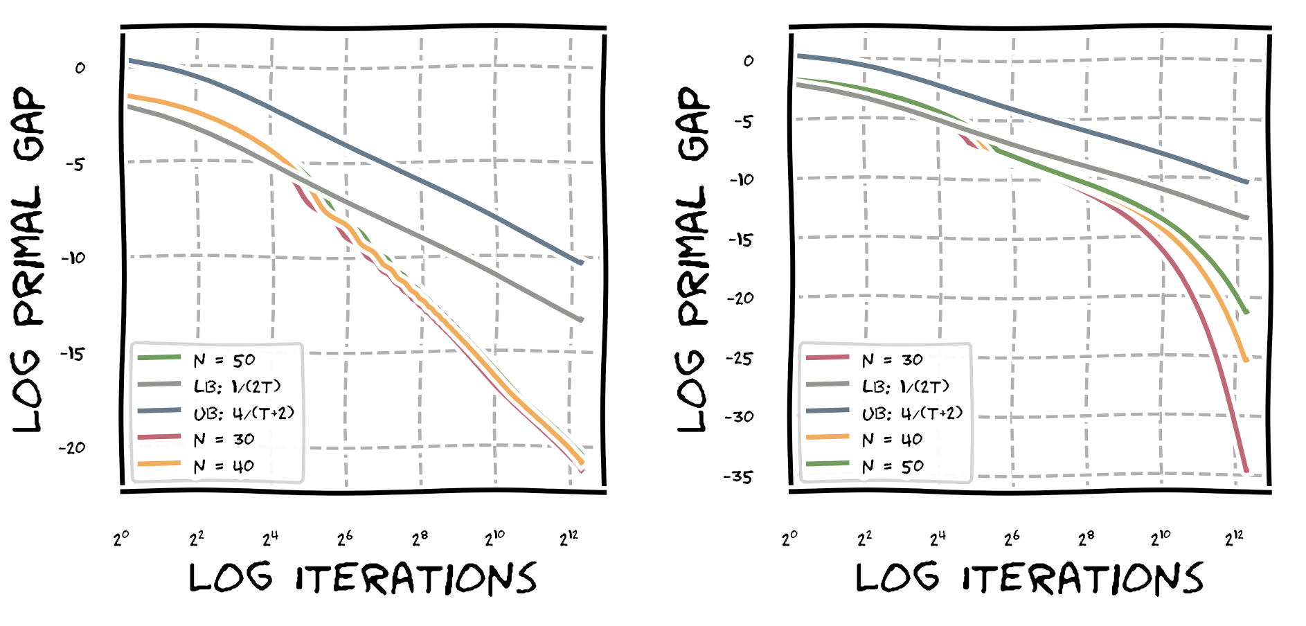
Hence we roughly have that the upper bound is an additive shift of the lower bound. Let us now look at actual computations. In the figure below we depict the convergence of the standard Frank-Wolfe algorithm using the step size rule $\gamma_t = \frac{\langle \nabla f(x_{t-1}), x_{t-1} - v_t \rangle}{L}$, where $v_t$ is the Frank-Wolfe vertex of the respective round; this is the analog of the short step for Frank-Wolfe (see last post). We depict convergence on probability simplices of sizes $n \in \setb{30,40,50}$ as well as the upper bound function $\operatorname{ub(t)} \doteq \frac{4}{t+2}$ and the lower bound function $\operatorname{lb(t)} \doteq \frac{1}{2t}$. On the left, we see the first $100$ iterations only and then on the right the first $5000$ iterations. It is important to note that we plot the primal gap $h(x_t)$ here and not the primal function value $f(x_t)$.

Convergence for different simplices

As we can see, for all three instances the primal gaps stay neatly within the upper and lower bound but then suddenly, they break out, below the lower bound curve and we can see from the plot that the primal gaps drops super-polynomially fast. To avoid confusion, keep in mind that we only established the validity of the lower bound up to $\lfloor n/2 \rfloor$ iterations, where $n$ is the dimension of the simplex. Now let us us have a closer look what is really happening. In the next graph we only consider the instance $n=30$ for the first $200$ iterations.

Three regimes

We have three distinct regimes. In regime $R_1$ for $t \in [1, n/2]$, we see that $\operatorname{lb(t)} \leq h(x_t) \leq \operatorname{ub(t)}$. In the second regime $R_2$ for $t \in [n/2 + 1, n]$, we see that $h(x_t)$ crosses the lower bound and we can also see that in regimes $R_1$ and $R_2$ we have that $h(x_t)$ drops super-polynomially. Then for $t = n$, where regime $R_3$ begins the convergence rate abruptly slows down, however it continues to drop super-polynomially as we have seen in the graphs above.

Quantifying convergence

Next, let us try to put some actual numbers, beyond intuition, to what is happening in our example. For the sake of exposition we will favor simplicity over sharpness of the derived rates. In fact the obtained rates are not optimal as we can see by comparing them to the figures above. Recall the definition of strong convexity:

Definition (strong convexity). A convex function $f$ is said to be $\mu$-strongly convex if for all $x,y \in \mathbb R^n$ it holds: $f(y) - f(x) \geq \nabla f(x)(y-x) + \frac{\mu}{2} \| x-y \|^2$.

For the analysis we will need the following bound on the primal gap induced by strong convexity:

\[f(x_t) - f(x^\esx) \leq \frac{\langle\nabla f(x_t),x_t - x^\esx\rangle^2}{2 \mu \norm{x_t - x^\esx}^2},\]

as well as the progress induced by smoothness (using e.g., the short step rule):

\[f(x_{t}) - f(x_{t+1}) \geq \frac{\langle \nabla f(x_t), d\rangle^2}{2L \norm{d}^2},\]

where $d$ is some direction that we consider (see last post for both derivations). If we could now (non-deterministcally) choose $d \doteq x_t - x^\esx$, then we immediately can combine these two inequalities to combine:

\[f(x_{t}) - f(x_{t+1}) \geq \frac{\mu}{L} h(x_t),\]

and iterating this inequality we obtain linear convergence. However, in fact, usually we do not have access to $d \doteq x_t - x^\esx$, so that we somehow have to relate the step that we take, i.e., the Frank-Wolfe step to this “optimal” direction. In fact, to simplify things we will relate the Frank-Wolfe step to $\norm{\nabla f(x_t)}$ and then use that $\langle \nabla f(x_t), \frac{x_t - x^\esx}{\norm{x_t - x^\esx}}\rangle \leq \norm{\nabla f(x_t)}$ by Cauchy-Schwartz. In particular, we want to show that there exists $1 \geq \alpha > 0$, so that

\[\begin{align} f(x_{t}) - f(x_{t+1}) & \geq \frac{\langle \nabla f(x_t), x_t - v \rangle^2}{2L \norm{x_t - v}^2} \\ & \geq \alpha^2 \frac{\norm{\nabla f(x_t)}^2}{2L} \\ & \geq \alpha^2 \frac{\langle \nabla f(x_t), x_t - x^\esx \rangle^2}{2L \norm{x_t - x^\esx}^2}, \end{align}\]

by means of showing $\frac{\langle \nabla f(x_t), x_t - v \rangle}{\norm{x_t - v}} \geq \alpha \norm{\nabla f(x_t)}$. We can then complete the argument as before simply losing the multiplicative factor $\alpha^2$ and obtain:

\[f(x_{t}) - f(x_{t+1}) \geq \alpha^2 \frac{\mu}{L} h(x_t),\]

or equivalently,

\[h(x_{t+1}) \leq \left(1 - \alpha^2 \frac{\mu}{L}\right) h(x_t).\]

To get slightly sharper bounds, we can estimate $\alpha$ separately in each iteration, which we will do now:

Observation. For $t \leq n$ the scaling factor $\alpha_t$ satisfies $\alpha_t \geq \sqrt{\frac{1}{2t}}$.

Proof. Our starting point is the inequality $\frac{\langle \nabla f(x_t), x_t - v \rangle}{\norm{x_t - v}} \geq \alpha_t \norm{\nabla f(x_t)}$, for which we want to determine a suitable $\alpha_t$. Observe that for $f(x) = \norm{x}^2$, we have $\nabla f(x) = 2x$. Thus the inequality becomes \[ \frac{\langle 2 x_t, x_t - v \rangle}{\norm{x_t - v}} \geq \alpha_t \norm{2 x_t}. \] Now observe that if we pick $v = \arg \max_{x \in P} \langle \nabla f(x_t), x_t - v \rangle$, then for rounds $t \leq n$, there exists a least one base vector $e_i$ that is not yet in the support of $x_t$ (where the support is simple set of the vertices in the convex combination that convex combine $x_t$), so that $\langle x_t, v \rangle = 0$. Thus the above can be further simplified to \[ \frac{2 \norm{x_t}^2}{\norm{x_t - v}} \geq \alpha_t 2 \norm{ x_t} \quad \Leftrightarrow \quad \frac{\norm{x_t}}{\norm{x_t - v}} \geq \alpha_t. \] Moreover, $\norm{x_t}\geq \sqrt{\frac{1}{t}}$ and $\norm{x_t - v} \leq \sqrt{2}$, so that we obtain a choice $\alpha_t \doteq \sqrt{\frac{1}{2t}}$. \[\qed\]

Combining this with the above, recalling that $L = \mu = 2$ in our example, we obtain up to iteration $t\leq n$, a contraction of the form

\[h(x_n) \leq h(x_0) \prod_{t = 2}^n \left(1-\alpha_t^2\right) = h(x_0) \prod_{t = 2}^n \left(1-\frac{1}{2t}\right) \leq \prod_{t = 2}^n \left(1-\frac{1}{2t}\right),\]

as $h(x_0) \leq 1$. In fact I strongly suspect that the $2$ in the above can be shaved off as well, as then we would obtain a contraction of the form:

\[\tag{estimatedConv} h(x_n) \leq \prod_{t = 2}^n \left(1-\frac{1}{t}\right) = \frac{1}{n},\]

which would be in line with the observed rates in the following graphic. The factor $2$ that arose from estimating $\norm{x_t -v} \leq \sqrt{2}$ can be at least partially improved, in particular if we would use line-search, this would actually reduce to $\norm{x_t -v } = \sqrt{1+ \frac{1}{t}}$ and the short step rule should be pretty close to the line search step as $f$ is actually a quadratic (might update the computation at a later time to see whether this can be made precise). Assuming that we are “close enough” to the line search guarantee of $\norm{x_t -v } = \sqrt{1+ \frac{1}{t}}$, we obtain the desired bound as now

\[ \alpha_t \leq \sqrt{\frac{1}{t+1}} = \sqrt{\frac{1}{t (1+ \frac{1}{t})}} \leq \frac{\norm{x_t}}{\norm{x_t - v}}, \]

and we can choose $\alpha_t \doteq \sqrt{\frac{1}{t+1}}$, so that

\[h(x_n) \leq h(x_0) \prod_{t = 2}^n \left(1-\alpha_t^2\right) = h(x_0) \prod_{t = 2}^n \left(1-\frac{1}{t+1}\right) \leq \prod_{t = 2}^n \left(1-\frac{1}{t+1}\right),\]

where the $t+1$ vs. $t$ offset is due to index shifting and we obtain the desired form (estimatedConv); in the worst-case within a factor of $2$.

Note, in the following graph the upper bound is now $1/t$ as function of $t$ and lower bound is $1/t - 1/n$ plotted for $n=30$ as a function of $t$. Clearly, the lower bound is only valid for $t\leq n$. Again we depict two regimes: left for the first $200$ iterations, right for the first $2000$ iterations.

Linear vs. Sublinear Convergence

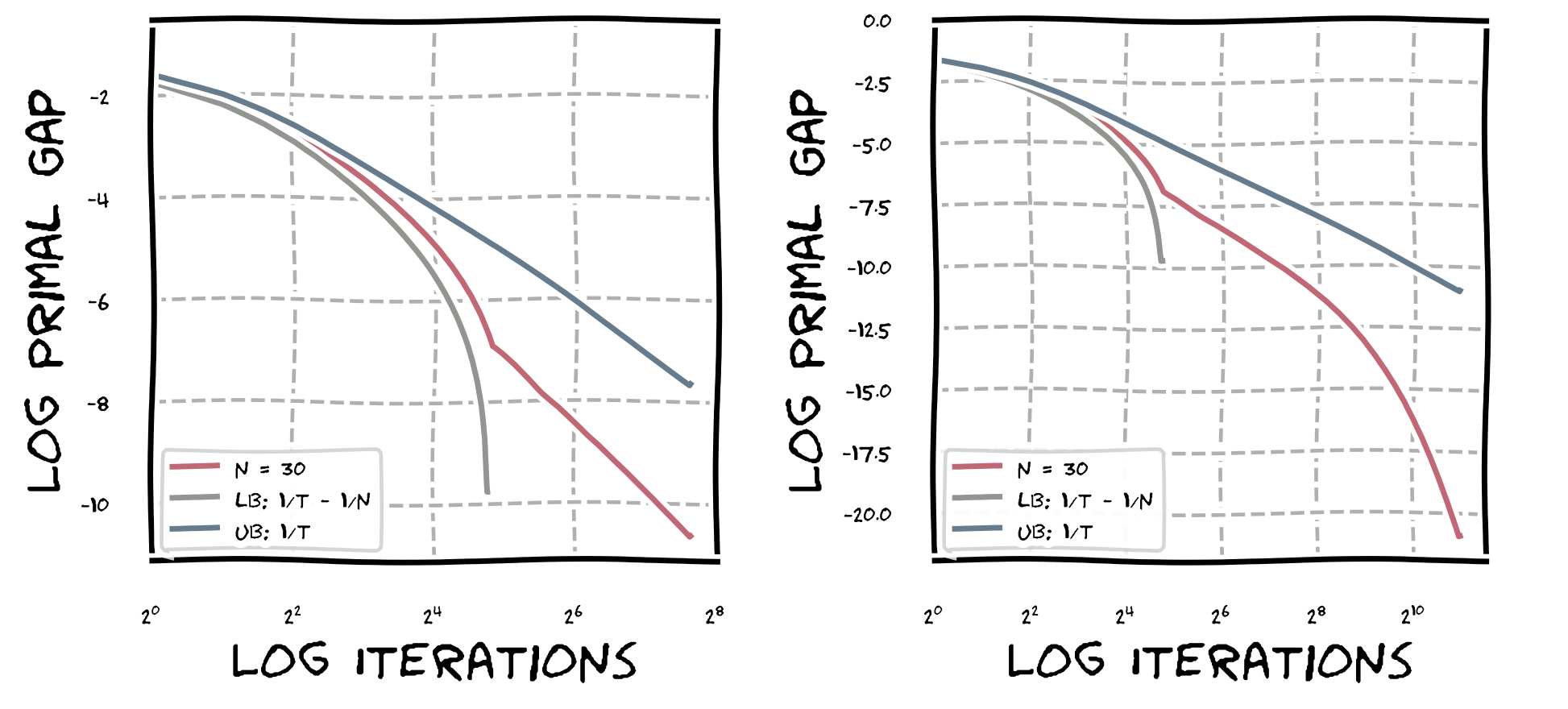
In fact, after closer inspection, it seems that locally we are actually doing slightly better than $\alpha_t = \sqrt{\frac{1}{t}}$, but for the sake of argument of linear convergence we could safely estimate $\alpha_t \geq \sqrt{\frac{1}{2n}}$ to show linear convergence up to $t \leq n$; as a side note, we can always do this: bounding the progress with the worst-case progress per round and calling it “linear convergence”. The key however is that we can show that there is a reasonable lower bound independent of $\varepsilon > 0$.

To this end, we will now analyze the sudden change of slope for $t > n$ and we will show that even after that change of slope, we still have a reasonable lower bound for the $\alpha_t$ independent of $t$ or $\varepsilon$. Intuitively, the sudden change in slope makes sense: from iteration $t+1$ onwards we cannot use $\langle x_t, v \rangle = 0$ anymore as all vertices have been picked up and the estimation from above gets much weaker. However, we will see now that we can still bound $\norm{\nabla f(x_t)}$ in a similar fashion; this argument is originally due to [GM] and we will revisit it in isolated and more general form in the next section.

Observation. There exists $t’ \geq n$ so that for all $t \geq t’$ the scaling factor $\alpha_t$ satisfies $\alpha_t \geq \sqrt{\frac{1}{8n}}$.

Proof. Suppose that we are in iteration $t > n$ and let $H$ be the affine space that contains $P$. Suppose that there exists a ball $B(x^\esx, 2 r ) \cap H \subseteq P$ of radius $2r$ around the optimal solution that is contained in the relative interior of $P$. If now the primal gap $h(x_{t’}) \leq r^2$ for some $t’$, it follows by smoothness $\norm{x_{t} - x^\esx}^2 \leq h(x_{t}) \leq h(x_{t’}) \leq r^2$ for $t \geq t’$, as $h(x_t)$ is monotonously decreasing (by the choice of the short step) and $L=2$. Thus for $t \geq t’$ it holds $\norm{x_t - x^\esx} \leq r$. For the remainder of the argument let us assume that the gradient $\nabla f(x_t)$ is already projected onto the linear space $H$. Therefore $x_t + r \frac{\nabla f(x_t)}{\norm{\nabla f(x_t)}} \in B(x^\esx, 2 r ) \cap H \subseteq P$ and as such $d \doteq r \frac{\nabla f(x_t)}{\norm{\nabla f(x_t)}}$ is a valid direction and we have \[ \max_{x \in P} \langle \nabla f(x_t),x_t - v\rangle \geq \langle \nabla f(x_t), d\rangle = r \norm{\nabla f(x_t)}, \] and in particular \[ \frac{\langle \nabla f(x_t),x_t - v\rangle}{\norm{x_t - v}} \geq \frac{r}{\norm{x_t - v}} \norm{\nabla f(x_t)} \geq \frac{r}{\sqrt{2}} \norm{\nabla f(x_t)}. \] For the choice $r \doteq \frac{1}{2\sqrt{n}}$, we have $B(x^\esx, 2 r ) \cap H \subseteq P$, so that we obtain a choice of $\alpha_t \doteq \frac{1}{2\sqrt{2n}}$ and a contraction of the form \[ h(x_{t+1}) \leq h(x_t) \left(1 - \frac{1}{8n} \right). \] \[\qed\]

To finish off this exercise, let us briefly derive a lower bound for any linear rate. To this end, recall that $h(x_{n/2}) \geq 1/n$. Moreover, we have $h(x_0) \leq 1$. Suppose we have a linear rate with constant $\beta$, then

\[\frac{1}{n} \leq h(x_0) \left(1-\beta\right)^{n/2} \leq \left(1-\beta\right)^{n/2},\]

and as such we have $- \ln n \leq (n/2) \ln(1-\beta)$ or equivalently

\[- \frac{2 \ln n}{n} \leq \ln (1 - \beta) \leq - \beta,\]

so that $\beta \leq \frac{2 \ln n}{n}$ follows, or put differently, any linear rate has to depend on the dimension $n$.

Impact of the step size rule

For completeness, the step size rule is important to achieve linear convergence. In particular, the standard Frank-Wolfe step size rule of $\frac{2}{t+2}$ does not induce linear convergence, as we can see in the graph below. On the left is the standard Frank-Wolfe step size rule and the right the short step rule from above for comparison. The key difference is that the short step rule roughly maximizes progress via the smoothness equation. Note, however that from the graph we can see the standard Frank Wolfe step size rule still does induce a convergence rate of $O(1/\varepsilon^p)$ for some $p > 1$, i.e., outperforming $O(1/\varepsilon)$ convergence for iterations $t \geq n$.

Comparison different step size rules

Linear Convergence for Frank-Wolfe

After having worked through the example to hopefully get some intuition what is going on, let us no turn to the general setup. We consider the problem:

\[\min_{x \in P} f(x), \tag{P}\]

where $P$ is a polytope and $f$ is a strongly convex function. Note that we restrict ourselves to polytopes here not merely for exposition but because the involved quantities that we will need are only defined for the polyhedral case and in fact these quantities can approach $0$ for general compact convex sets.

Before we consider the general setup, observe that the arguments in the example above do not cleanly separate out the contribution of the geometry from the contribution of the strong convexity of the function. While this helped a lot with simplifying the arguments, this is highly undesirable and we will work towards a clean separation of the contribution of strong convexity of the function and the contribution of the geometry of the polytope towards the rate of linear convergence. Ultimately, we have already seen what we have to show for the general case: there exists $\alpha > 0$, so that for any iterate $x_t$, our algorithms (Frank-Wolfe or modifications of such) provide a direction $d$, so that

\[\frac{\langle \nabla f(x_t), d \rangle}{\norm{d}} \geq \alpha \frac{\langle \nabla f(x_t), x_t - x^\esx \rangle}{\norm{x_t - x^\esx}}. \tag{Scaling}\]

This condition should serve as a guide post throughout the following discussion: if such an $\alpha$ exists, we basically obtain a linear rate of $\alpha^2 \frac{\mu}{L}$, i.e., $h(x_t) \leq h(x_0) \left(1- \alpha^2 \frac{\mu}{L}\right)^t$, exactly as done above.

The simple case: $x^\esx$ in strict relative interior

In the example above we have actually proven something stronger, which is due to [GM] (and holds more generally for compact convex sets):

Theorem (Linear convergence for $x^\esx$ in relative interior [GM]). Let $f$ be a smooth strongly convex function with smoothness $L$ and strong convexity parameter $\mu$. Further let $P$ be a compact convex set. If $B(x^\esx,2r) \cap \operatorname{aff}(P) \subseteq P$ with $x^\esx \doteq \arg\min_{x \in P} f(x)$ for some $r > 0$, then there exists $t’$ such that for all $t \geq t’$ it holds \[ h(x_t) \leq \left(1 - \frac{r^2}{D^2} \frac{\mu}{L}\right)^{t-t’} h(x_{t’}), \] where $D$ is the diameter of $P$ with respect to $\norm{\cdot}$.

Proof. We basically gave the proof above already. The key insight is that if $x^\esx$ is contained $2r$-deep in the relative interior, then we can show the existence of some $t’$ so that for all $t\geq t’$ it holds \[ \frac{\langle \nabla f(x_t),x_t - v\rangle}{\norm{x_t - v}} \geq \frac{r}{D} \norm{\nabla f(x_t)}. \] and then we plug this into the formula from the example with $\alpha = \frac{r}{D}$. $\qed$

The careful reader will have observed that in the example as well as in the proof above, we realize a bound

\[\frac{\langle \nabla f(x_t), d \rangle}{\norm{d}} \geq \alpha \norm{\nabla f(x_t)},\]

which is stronger than what (Scaling) requires, using $\frac{\langle \nabla f(x_t), x_t - x^\esx \rangle}{\norm{x_t - x^\esx}} \leq \norm{\nabla f(x_t)}$. This stronger condition cannot be satisfied in general: if $x^\esx$ lies on the boundary of $P$, then $\norm{\nabla f(x_t)}$ does not vanish (while $\langle \nabla f(x_t), x_t - x^\esx \rangle$ does) and therefore this condition is unsatisfiable as it would guarantee infinite progress via smoothness. This is not the only problem though as we could directly aim for establishing (Scaling). However, it turns out that the standard Frank-Wolfe algorithm cannot achieve linear convergence when the optimal solution $x^\esx$ lies on the (relative) boundary of $P$, as the following theorem shows:

Theorem (FW converges sublinearly for $x^\esx$ on the boundary [W]). Suppose that the (unique) optimal solution $x^\esx$ lies on the boundary of the polytope $P$ and is not an extreme point of $P$. Further suppose that there exists an iterate $x_t$ that is not already contained in the same minimal face as $x^\esx$. Then for any $\delta > 0$ constant, the relation \[ f(x_t) - f(x^\esx) \geq \frac{1}{t^{1+\delta}}, \] holds for infinitely many indices $t$.

Introducing Away-Steps

So what is the fundamental reason that we cannot achieve basically better than $\Omega(1/t)$-rates if $x^\esx$ is on the boundary? The problem lies in the scaling condition that we want to satisfy via Frank-Wolfe steps, i.e.,

\[\frac{\langle \nabla f(x_t), x_t - v \rangle}{\norm{x_t - v}} \geq \alpha \frac{\langle \nabla f(x_t), x_t - x^\esx \rangle}{\norm{x_t - x^\esx}}.\]

The closer we get to the boundary the smaller $\langle \nabla f(x_t), x_t - v \rangle$ gets: the direction $\frac{x_t - v}{\norm{x_t - v}}$ approximates the gradient $\nabla f(x_t)$ worse and worse compared to the direction $\frac{x_t - x^\esx}{\norm{x_t - x^\esx}}$. This is basically also how the proof of the theorem above works: we need that $x^\esx$ is not an extreme point, otherwise for $x^\esx = v$ the approximation cannot be arbitrarily bad and at no point do we need to be in the face of the optimal solution as otherwise we are back to the case of the relative interior. As a result of this flattening of the gradient approximations we observe the (relatively well-known) zig-zagging phenomenon (see figure further below).

The ultimate reason for the zig-zagging is that we lack directions in which we can go that guarantee (Scaling). The first ones to overcome this challenge in the general case were Garber and Hazan [GH]. At the risk of oversimplifying their beautiful result, the main idea to define a new oracle that does not perform linear optimization over $P$ but over $P \cap \tilde B(x_t,\varepsilon)$, some notion of “ball”, so that $p = \arg \min_{P \cap \tilde B(x_t,\varepsilon)} \nabla f(x_t)$, produces a point $p \in P$ (usually not a vertex), so that the direction

\[\frac{\langle \nabla f(x_t), x_t - d \rangle}{\norm{x_t - d}} \geq \alpha \frac{\langle \nabla f(x_t), x_t - x^\esx \rangle}{\norm{x_t - x^\esx}}.\]

is satisfied for some $\alpha$. This is “trivial” if $\tilde B$ is the euclidean ball as then $x_t - d = - \varepsilon \nabla f(x_t)$ if $\varepsilon$ is small enough; we are then basically in the case of the interior solution. The key insight in [GH] however is that you can define a notion of ball $\tilde B$, so that you can solve this modified oracle with a single call to the original LP oracle and still ensure (Scaling). What this really comes down to is that you add many more directions that ultimately provide better approximations of $\frac{\langle \nabla f(x_t), x_t - x^\esx \rangle}{\norm{x_t - x^\esx}}$. Unfortunately, the resulting algorithm is extremely hard to implement and not practical due to exponentially sized constants.

What we will consider in the following is an alternative approach to add more directions, which is due to [W]. Suppose we have an iterate $x_t$ obtained via a couple of Frank-Wolfe iterations. Then $x_t = \sum_{i \in [t]} \lambda_i v_i$, where $v_i$ with $i \in [t]$ are extreme points of $P$, $\lambda_i \geq 0$ with $i \in [t]$, and $\sum_{i \in [t]} \lambda_i = 1$. We call the set $\setb{v_i \mid \lambda_i > 0, i \in [t] }$ the active set $S_t$. So additionally to Frank-Wolfe directions of the form $x_t - v$, we can consider $a \doteq \arg\max_{v \in S} \nabla f(x_t)$ (as opposed to $\arg\min$ for Frank-Wolfe directions) and the resulting away direction $a - x_t$, that does not add a new vertex but removes weight from a previously added vertex; since we have the decomposition, we know exactly how much weight can be removed, while staying feasible. The reason why this is useful is that it not just adds some additional directions, but directions that intuitively make sense: Slow convergence happens because we cannot enter to optimal face that contains $x^\esx$ fast enough and this is because we have a vertex in the convex combination that keeps the iterates from reaching the face and with Frank-Wolfe steps we would now slowly wash out this blocking vertex (basically at a rate of $1/t$). An away step, which is following an away direction can potentially remove the same blocking vertex in a single iteration. Let us consider the following figure, where on the left we see the normal Frank-Wolfe behavior and on the right the behavior with an away step; in the example the depicted polytope is $\operatorname{conv}(S_t)$ (see [JL] for a nicer illustration).

Away-step of FW

With this improvement we can formulate:

Away-step Frank-Wolfe (AFW) Algorithm [W]
Input: Smooth convex function $f$ with first-order oracle access, feasible region $P$ with linear optimization oracle access, initial vertex $x_0 \in P$ and initial active set $S_0 = \setb{x_0}$.
Output: Sequence of points $x_0, \dots, x_T$
For $t = 0, \dots, T-1$ do:
$\quad v_t \leftarrow \arg\min_{x \in P} \langle \nabla f(x_{t}), x \rangle \quad \setb{\text{FW direction}}$
$\quad a_t \leftarrow \arg\max_{x \in S_t} \langle \nabla f(x_{t}), x \rangle \quad \setb{\text{Away direction}}$
$\quad$ If $\langle \nabla f(x_{t}), x_t - v_t \rangle > \langle \nabla f(x_{t}), a_t - x_t \rangle: \quad \setb{\text{FW vs. Away}}$
$\quad \quad x_{t+1} \leftarrow (1-\gamma_t) x_t + \gamma_t v_t$ with $\gamma_t \in [0,1]$ $\quad \setb{\text{Perform FW step}}$
$\quad$ Else:
$\quad \quad x_{t+1} \leftarrow (1+\gamma_t) x_t - \gamma_t a_t$ with $\gamma_t \in [0,\frac{\lambda_{a_t}}{1-\lambda_{a_t}}]$ $\quad \setb{\text{Perform Away step}}$
$\quad S_{t+1} \rightarrow \operatorname{ActiveSet}(x_{t+1})$

In the above $\lambda_{a_t}$ is the weight of vertex ${a_t}$ in decomposition of $x_t$ in iteration $t$. Moreover, by the same smoothness argument as we have used now multiple times, the progress of an away step, provided it did not hit the upper bound $\frac{\lambda_{a_t}}{1-\lambda_{a_t}}$, is at least

\[f(x_t) - f(x_{t+1}) \geq \frac{\langle \nabla f(x_{t-1}), a_t - x_t \rangle^2}{2L \norm{a_t - x_t}},\]

i.e., the same type of progress that we have for the FW steps. If we hit the upper bound then vertex $a_t$ is removed from the convex combination / active set and we call this a drop step.

Observation (A case for FW). We will see in the next section that the Away-step Frank-Wolfe algorithm achieves linear convergence (for strongly convex functions) even for optimal solutions on the boundary. Moreover, it has been widely empirically observed that AFW has better per-iteration convergence than FW. So irrespective of the convergence rate proof, why not always using the AFW variant given that the additional computational overhead is small? In some cases the vanilla FW can have a huge advantage over the AFW: it does not have to maintain the active set for the decomposition and for some problems, e.g., matrix completion this matters a lot. For example some of the experiments in [PANJ] could not be performed for variants other than FW that need to maintain the active set. Now, there are special cases (see, e.g., [GM2]) or when assuming the existence of a rather strong away oracle (see, e.g., [BZ]) that we do not need to maintain active sets. For completeness and slightly simplifying, what the away oracle does, it solves $\max_{x \in P \cap F} \nabla f(x_t)$, where $F$ is the minimal face that contains $x_t$. One can then easily verify that the optimal solution is an away vertex for some decomposition of $x_t$ and in fact it will induce the largest progress (provided it is not a drop step); see [BZ] for details.

Pyramidal width and linear convergence for AFW

So how do we obtain linear convergence with the help of away steps? The key insight here is due to Lacoste-Julien and Jaeggi [LJ] that showed that there exists a geometric constant $w(P)$, the so-called pyramidal width that only depends on the polytope $P$. While the full derivation of the pyramidal width would be very tedious, it provides the following crucial strong convexity bound:

\[h(x_t) \leq \frac{\langle \nabla f(x_{t}), a_t - v_t \rangle^2}{2 \mu w(P)^2},\]

where $\mu$ is the strong convexity constant of the function $f$. If we plug this back into the standard progress equation (as done before), we obtain:

\[h(x_{t+1}) \leq h_t \left(1 - \frac{\mu}{L} \frac{w(P)^2}{D^2} \right),\]

where $D$ is the diameter of $P$, i.e., we obtain linear convergence. Note, that I have cheated slightly here not accounting for the drop steps (no more than genuine FW steps). Rephrasing the provided bound into our language here (see Theorem’ 3 in [LJ]), it holds:

\[\langle \nabla f(x_{t}), a_t - v_t \rangle \geq w(P) \frac{\langle \nabla f(x_t), x_t - x^\esx \rangle}{\norm{x_t - x^\esx}},\]

where the missing term $\norm{a_t - v_t}$ can be absorbed in various way, e.g., bounding it via the diameter $D$ of $P$ (that is where the $D^2$ term above comes from), absorbing into $w(P)$ itself, or absorbing it into the definition of curvature in the case of the affine-invariant version of AFW, so that we obtain (Scaling) again and we can use a line of arguments as above to complete the proof. Here we assume that would do either an away step or a Frank-Wolfe were at least one of them has to recover $1/2$ of $\langle \nabla f(x_{t}), a_t - v_t \rangle$, i.e., either

\[\langle \nabla f(x_{t}), x_t - v_t \rangle \geq 1/2 \ \langle \nabla f(x_{t}), a_t - v_t \rangle\]

\[\langle \nabla f(x_{t}), a_t - x_t \rangle \geq 1/2 \ \langle \nabla f(x_{t}), a_t - v_t \rangle.\]

Final comments

I would like to end this post with a few comments:

The Away-step Frank-Wolfe algorithm can be further improved by not choosing either a FW step or an Away step but by directly combining those into a direction $d \doteq a_t - v_t$, which leads to the Pairwise Conditional Gradients algorithm, which is typically faster but harder to analyze due to so called swap steps, when one vertex leaves the active sets and another one enters at the same time.
Recently, in [PR] and [GP], the notion of pyramidal width has been further simplified and generalized.
There is also a very beautiful way of achieving (Scaling) in the decomposition-invariant case where no active set has to be maintained. The initial key insight here is due to [GM2], where they show that if $\norm{x_t - x^\esx}$ is small, then so is the amount of weight that needs to be shifted around in the convex combination of $x_t$ to represent $x^\esx$. This can then be directly combined with the away steps to obtain (Scaling). In [GM2] the construction works for certain structured polytopes only and this has been recently extended in [BZ] to the general case.

References

[CG] Levitin, E. S., & Polyak, B. T. (1966). Constrained minimization methods. Zhurnal Vychislitel’noi Matematiki i Matematicheskoi Fiziki, 6(5), 787-823. pdf

[FW] Frank, M., & Wolfe, P. (1956). An algorithm for quadratic programming. Naval research logistics quarterly, 3(1‐2), 95-110. pdf

[J] Jaggi, M. (2013, June). Revisiting Frank-Wolfe: Projection-Free Sparse Convex Optimization. In ICML (1) (pp. 427-435). pdf

[GM] Guélat, J., & Marcotte, P. (1986). Some comments on Wolfe’s ‘away step’. Mathematical Programming, 35(1), 110-119. pdf

[W] Wolfe, P. (1970). Convergence theory in nonlinear programming. Integer and nonlinear programming, 1-36.

[GH] Garber, D., & Hazan, E. (2013). A linearly convergent conditional gradient algorithm with applications to online and stochastic optimization. arXiv preprint arXiv:1301.4666. pdf

[PANJ] Pedregosa, F., Askari, A., Negiar, G., & Jaggi, M. (2018). Step-Size Adaptivity in Projection-Free Optimization. arXiv preprint arXiv:1806.05123. pdf

[GM2] Garber, D., & Meshi, O. (2016). Linear-memory and decomposition-invariant linearly convergent conditional gradient algorithm for structured polytopes. In Advances in Neural Information Processing Systems (pp. 1001-1009). pdf

[BZ] Bashiri, M. A., & Zhang, X. (2017). Decomposition-Invariant Conditional Gradient for General Polytopes with Line Search. In Advances in Neural Information Processing Systems (pp. 2690-2700). pdf

[LJ] Lacoste-Julien, S., & Jaggi, M. (2015). On the global linear convergence of Frank-Wolfe optimization variants. In Advances in Neural Information Processing Systems (pp. 496-504). pdf

[PR] Pena, J., & Rodriguez, D. (2018). Polytope conditioning and linear convergence of the Frank–Wolfe algorithm. Mathematics of Operations Research. pdf

[GP] Gutman, D. H., & Pena, J. F. (2018). The condition of a function relative to a polytope. arXiv preprint arXiv:1802.00271. pdf