Cheat Sheet: Frank-Wolfe and Conditional Gradients

TL;DR: Cheat Sheet for Frank-Wolfe and Conditional Gradients. Basic mechanics and results; this is a rather long post and the start of a series of posts on this topic.

Posts in this series (so far).

My apologies for incomplete references—this should merely serve as an overview.

One of my favorite topics that I am currently interested in is constraint smooth convex optimization and in particular projection-free first-order methods, such as the Frank-Wolfe Method [FW] aka Conditional Gradients [CG]. In this post, I will provide a basic overview of these methods, how they work, and my perspective which will be the basis for some of the future posts.

The goal: Smooth Constraint Convex Minimization

The task that we will be considering here is to solve constrained smooth convex optimization of the form

\[\min_{x \in P} f(x),\]

where $f$ is a differentiable convex function, $P$ is some compact and convex feasible region; you might want to think of $P$, e.g., being a polytope, which is one of the most common cases. As such, for the sake of exposition we will assume that $P \subseteq \mathbb R^n$ is a polytope. We are interested in general purpose methods and not methods specialized to specific problem configurations.

First, we need to agree on how we can access the function $f$ and the feasible region $P$. For the feasible region $P$ we assume access by means of a so-called linear programming oracle:

Linear Programming oracle
Input: $c \in \mathbb R^n$
Output: $\arg\min_{x \in P} \langle c, x \rangle$

We further assume that we can access $f$ by means of a so-called first-order oracle:

First-Order oracle
Input: $x \in \mathbb R^n$
Output: $\nabla f(x)$ and $f(x)$

Many problems of interest in optimization and machine learning can be naturally cast in this setting, such as, e.g., Linear Regression with LASSO:

Example: LASSO Regression
Linear Regression with LASSO regularization can be formulated as minimizing a quadratic loss function over a (rescaled) $\ell_1$-ball: $\min_{\beta, \beta_0} \{\frac{1}{N} \|y- \beta_0 1_N - X\beta\|_2^2 \ \mid \ \|\beta\|_1 \leq t\}.$

The workhorses: convexity and smoothness

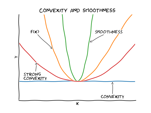
In smooth convex optimization we have two key concepts (and variations of those) that drive most results: smoothness and convexity.

Convexity provides an under-estimator for the change of the function $f$ by means of a linear function, actually the Taylor-expansion first-order estimation.

Definition (convexity). A differentiable function $f$ is said to be convex if for all $x,y \in \mathbb R^n$ it holds: $f(y) - f(x) \geq \nabla f(x)(y-x)$.

Smoothness provides an over-estimator of the change of the function $f$ by means of a quadratic function; in fact the smoothness inequality works in reverse compared to convexity. For the sake of simplicity we will work with the affine-variant versions however similar affine-invariant versions exist.

Definition (smoothness). A convex function $f$ is said to be $L$-smooth if for all $x,y \in \mathbb R^n$ it holds: $f(y) - f(x) \leq \nabla f(x)(y-x) + \frac{L}{2} \| x-y \|^2$.

Finally, we have strong convexity, which provides provides a quadratic under-estimator for the change of the function $f$, again obtained from the Taylor-expansion. We will not exploit strong convexity today, except for the warm-up below, but it is helpful for understanding the overall context. Note that strong convexity is basically the reverse inequality of smoothness (and provides stronger bounds than simple convexity).

Definition (strong convexity). A convex function $f$ is said to be $\mu$-strongly convex if for all $x,y \in \mathbb R^n$ it holds: $f(y) - f(x) \geq \nabla f(x)(y-x) + \frac{\mu}{2} \| x-y \|^2$.

The following graphic relates the various concepts with each other:

Convexity and smoothness

Warmup: Gradient Descent from smoothness and (strong) convexity

As a warmup we will now establish convergence of gradient descent in the smooth unconstrained case. An important consequence of smoothness is that we can use it to lower bound the progress of a typical gradient step. Let $x_t \in \mathbb R^n$ be an (arbitrary) point and let $x_{t+1} = x_t - \eta \cdot d$, where $d \in \mathbb R^n$ is some direction. Using smoothness we obtain:

\[\underbrace{f(x_{t}) - f(x_{t+1})}_{\text{primal progress}} \geq \eta \langle\nabla f(x_t),d\rangle - \eta^2 \frac{L}{2} \|d\|^2\]

Optimizing the right-hand side for $\eta$ leads to $\eta^* = \frac{\langle\nabla f(x_t),d\rangle}{L \norm{d}^2}$, which upon plugging back in into the above, with the usual choice $d \doteq \nabla f(x_t)$, leads to:

Progress induced by smoothness: \[ \begin{equation} \underbrace{f(x_{t}) - f(x_{t+1})}_{\text{primal progress}} \geq \frac{\norm{\nabla f(x_t)}^2}{2L}. \end{equation} \]

We will first complete the argument using strong convexity now as it is significantly simpler than using convexity only. While smoothness provides a lower bound on the primal progress of a typical gradient step, we can use strong convexity to obtain an upper bound on the primal optimality gap $h(x_t) \doteq f(x_t) - f(x^*)$ by means of the norm of the gradient. The argument is very similar to the argument employed for the progress bound induced by smoothness. We start from the strong convexity inequality and apply it to the points $x = x_t$ and $y = x_t - \eta e_t$, where $e_t \doteq x_t - x^\esx$ is the direction pointing towards the optimal solution $x^*$; note that in the case of strong convexity the latter is unique. We have:

\[f(x_t - \eta e_t) - f(x_t) \geq - \eta \langle\nabla f(x_t),e_t\rangle + \eta^2\frac{\mu}{2} \| e_t \|^2.\]

If we now minimize the right-hand side of the above inequality over $\eta$, with an argument identical to the ones above the minimum is achieved for the choice $\eta^\esx \doteq \frac{\langle\nabla f(x_t), e_t\rangle}{\mu \norm{e_t}^2}$; note that is has the same form as the $\eta^*$ we derived via smoothness, however this time the inequality is reversed. Plugging this back in, we obtain

\[f(x_t) - f(x_t - \eta e_t) \leq \frac{\langle\nabla f(x_t),e_t\rangle^2}{2 \mu \norm{e_t}^2},\]

and as the right-hand side is now independent of $\eta$ we can choose $\eta = 1$ and observe that $\frac{\langle\nabla f(x_t),e_t\rangle^2}{\norm{e_t}^2} \leq \norm{\nabla f(x_t)}^2$, via the Cauchy-Schwarz inequality. We arrive at the actual upper bound from strong convexity that we care for.

Upper bound on primal gap induced by strong convexity: \[ \begin{equation} f(x_t) - f(x^\esx) \leq \frac{\norm{\nabla f(x_t)}^2}{2 \mu}. \end{equation} \]

From these two bounds we immediately obtain linear convergence in the case of strongly convex functions: We have $f(x_{t}) - f(x_{t+1}) \geq \frac{\mu}{L} (f(x_t) - f(x^\esx)),$ i.e., in each iteration we recover a $\mu/L$-fraction of the residual primal gap. Simply adding $f(x^\esx)$ on both sides and rearranging gives the desired bound per iteration

\[f(x_{t+1}) - f(x^\esx) \leq \left(1-\frac{\mu}{L}\right)(f(x_t) - f(x^\esx)),\]

which we iterate to obtain

\[f(x_T) - f(x^\esx) \leq \left(1-\frac{\mu}{L}\right)^T(f(x_0) - f(x^\esx)).\]

If we have only smooth and not necessarily strongly convex function the last part of the argument changes a little. Rather than plugging in the bound from strong convexity, we use convexity and estimate:

\[f(x_t) - f(x^\esx) \leq \langle \nabla f(x_t) , x_t - x^\esx \rangle \leq \norm{\nabla f(x_t)} \norm{(x_t - x^*)}.\]

This estimation is much weaker as the one from strong convexity and if we plug this into the progress inequality we only obtain:

\[f(x_{t+1}) - f(x_{t}) \geq \frac{(f(x_t) - f(x^\esx))^2}{2L \, \norm{(x_t - x^*)}^2} \geq \frac{(f(x_t) - f(x^\esx))^2}{2L \, \norm{(x_0 - x^*)}^2},\]

where the last inequality is not immediate but also not terribly hard to show. Now with some induction one can show the standard rate of roughly

\[f(x_T) - f(x^\esx) \leq \frac{2L \, \norm{(x_0 - x^*)}^2}{T+4}.\]

We skip the details here as we will see a similar induction below for the Frank-Wolfe algorithm.

Projections and the Frank-Wolfe method

So far we have considered unconstrained smooth convex minimization in the example above. At first sight, in the constrained case, the situation does not dramatically change: as soon as we have constraints, then basically we have to augment the methods from above to ‘project back’ into the feasible region after each step (otherwise a gradient step might lead us outside out of the feasible region). To this end, let $P$ be a compact convex feasible region and $\Pi_P$ be an appropriate projection onto $P$, then we simply modify the iterates of our gradient descent scheme to be

\[x_{t+1} \leftarrow \Pi_P(x_t - \eta \nabla f(x_t)).\]

This projection can be performed relatively easily for some domains and norms, e.g., the simplex (probability simplex), the $\ell_1$-ball, the $\ell_2$-ball, and more general permutahedra. However, as soon as the projection problem is not that easy to solve anymore, than the projection that we need can give basically rise to another optimization problem that can be expensive to solve.

This is where the Frank-Wolfe algorithm [FW] or Conditional Gradients [CG] come into play as a projection-free first-order method for constraint smooth minimization and the way these algorithms do this is by maintaining feasibility of all iterates $x_t$ throughout by merely forming convex combinations of the current iterate and a new point $v \in P$. But before we talk more about the why-you-should-care factor, let us first have a look at the (most basic variant of the) algorithm:

Frank-Wolfe Algorithm [FW]
Input: Smooth convex function $f$ with first-order oracle access, feasible region $P$ with linear optimization oracle access, initial point (usually a vertex) $x_0 \in P$.
Output: Sequence of points $x_0, \dots, x_T$
For $t = 1, \dots, T$ do:
$\quad v_t \leftarrow \arg\min_{x \in P} \langle \nabla f(x_{t-1}), x \rangle$
$\quad x_{t+1} \leftarrow (1-\gamma_t) x_t + \gamma_t v_t$

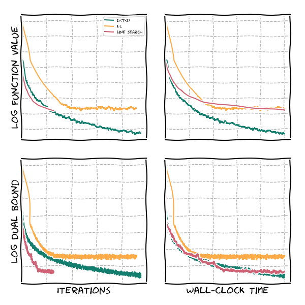
In the algorithm above the step size $\gamma_t$ can be set in various ways:

$\gamma_t = \frac{2}{t+2}$ (the original step size)
Assumes a worst-case upper bound on the function $f$. Does not require knowledge of $L$, although the convergence bound will depend on it. Does not ensure that we have monotonous progress. Basically, what this step size rule ensures is that $x_t$ is the uniform average of the vertices obtained up to that point from the linear optimization oracle.
$\gamma_t = \frac{\langle \nabla f(x_{t-1}), x_{t-1} -v_t \rangle}{L}$ (the short step; the analog to the above in the unconstrained case)
Approximately, minimizes the curvature equation as we have seen in the example above. Ensures monotone progress but requires approximate knowledge of $L$, or a search for it. Note that the magnitude of progress though does not have to be monotonous across iterations.
$\gamma_t$ via line search to maximize function decrease
Does not require any knowledge about $L$ and is also monotone, however requires several function evaluations to find the minimum. There has been some recent work on this specifically for Conditional Gradients algorithms that provides a reasonable tradeoff [PANJ].

The Frank-Wolfe algorithm has many appealing features. Just to name a few:

Extremely easy to implement
No complicated data structures to maintain, which makes it quite memory-efficient
No projections
Iterates are maintained as convex combinations. This can be useful when we interpret the final solution as a distribution over vertices.

Especially the last point is useful in many applications. Jumping slightly ahead, as we will prove below, for a general smooth convex function, the Frank-Wolfe algorithm achieves:

\[f(x_t) - f(x^\esx) \leq \frac{LD^2}{t+2} = O(1/t),\]

where $D$ is the diameter of $P$ in the used norm (in smoothness) and $L$ the Lipschitz constant from above.

Example: Approximate Carathéodory
Let $\hat x \in P$. Goal: find a convex combination $\tilde x$ of vertices of $P$, so that $\norm{\hat x-\tilde x} \leq \varepsilon$. This can be solved with the Frank-Wolfe algorithm via solving $\min_{x \in P} \norm{\hat x - x}^2$. We need an accuracy $\norm{\hat x - x}^2 \leq \varepsilon^2$, so that we roughly need $\frac{LD^2}{\varepsilon^2}$ iterations to achieve this approximation.
(For completeness: if we are willing to have a bound that explicitly depends on the dimension of $P$, then we can exploit the strong convexity of our objective and we need only roughly $O(n \log 1/\varepsilon)$ iterations. We will come back to the strongly convex case in a later post).

The following graph shows typical convergence of the Frank-Wolfe algorithm for the three step size rules above. As mentioned above, the step size rule $\frac{2}{t+2}$ does not guarantee monotonous progress. Moreover, as we can see for our choice of $L$ as a guess of the true Lipschitz constant, we converge to a suboptimal solution as $L$ was chosen (on purpose) to be too small. This is one of the main issues with estimated Lipschitz constants: when too small we might not converge. From the argumentation above in terms of progress one might be willing to opt for a much smaller guess but this immediately and strongly affects the progress: using $\alpha / L$ with $0 < \alpha < 1$ leads to an $\alpha$ slowdown. Also, note that while the $\frac{2}{t+2}$ rule makes less progress per iteration, in wall-clock time it is actually pretty fast here as we save on the function evaluations in the (admittedly simple) line search; one can do much better, see [PANJ]. We also depict a dual gap, which is upper bounding $f(x_t) - f(x^\esx)$ that we will explore in more detail in the next section.

FW Algorithm

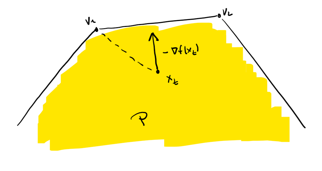
So what does the Frank-Wolfe algorithm actually do? As shown in the figure below, rather than using the negative gradient direction $-\nabla f(x_t)$ for descent, it uses a replacement direction $d = v - x_t$ with potentially weaker progress: $\frac{\norm{\nabla f(x_t)}^2}{2L}$ vs. $\frac{\langle{\nabla f(x_t),x_t-v\rangle}^2}{2LD^2}$. At the same time it is much easier to ensure feasibility for this direction as the next iterate $x_{t+1}$ is simply a convex combination of the current iterate $x_t$ and the vertex $v$ of $P$. Thus we do not have to do projection but we pay for this in (potentially) less progress per iteration—this is the tradeoff that Frank-Wolfe makes.

Convexity and smoothness

Dual gaps in constraint convex optimization

In the case of unconstrained gradient descent we had two types of dual gaps, i.e., those that bound $f(x_t) - f(x^\esx)$ as a function of the gradient. We will now obtain a similar dual gap that will be central to the Frank-Wolfe algorithm. Recall that we defined $h(x) \doteq f(x) - f(x^\esx)$ as the primal (optimality) gap $h(\cdot)$ above. In the context of constraint convex optimization we can define the following dual (optimality) gap $g(\cdot)$, which is often referred to as the Wolfe gap. To this end, observe that by convexity we have:

\[h_t = f(x) - f(x^\esx) \leq \langle \nabla f(x_t), x_t - x^\esx \rangle \leq \max_{x \in P} \langle \nabla f(x_t), x_t - x \rangle \doteq g(x_t).\]

There is two ways of thinking about the dual gap. First of all, it is upper bounding the primal gap, but also here we can understand $g(x_t)$ as computing the “best possible” approximation to $\nabla f(x_t)$. Of course, closer inspection reveals that this is flawed as stated, as it measures the quality of approximation scaled with the length of the line segment $x_t - x$:

\[g(x_t) = \max_{x \in P} \langle \nabla f(x_t), x_t - x \rangle = \max_{x \in P} \frac{\langle \nabla f(x_t), x_t - x \rangle}{\norm{x_t - x}} \cdot \norm{x_t - x}.\]

This subtlety is worth keeping in mind. Moreover, the dual gap also serves as an optimality certificate.

The Wolfe gap
We have $0 \leq h(x_t) \leq g(x_t)$. Moreover, $g(x) = 0 \Leftrightarrow f(x) - f(x^\esx) = 0$.

The proof of the above is straight forward: Clearly, if $g(x_t) = 0$, then $h(x_t) = 0$. For the converse, we go the lazy route through smoothness. We showed above that $f(x_{t}) - f(x_{t+1}) \geq \eta \langle\nabla f(x_t),d\rangle - \eta^2 \frac{LD^2}{2}$. In the case of Frank-Wolfe we have $d= v_t - x_t$ for the maximizing vertex $v_t$ as $x_{t +1} = (1-\gamma_t) x_t + \gamma_t v_t$. Choosing $\gamma_t = \min\setb{\frac{g(x_t)}{LD^2},1}$ yields:

\[f(x_t) - f(x_{t+1}) \geq \min\setb{g(x_t)/2,\frac{g(x_t)^2}{2LD^2}},\]

and since we were optimal the left-hand side is $0$. Thus $g(x_t) = 0$ follows.

Lemma (Frank-Wolfe convergence). After $t$ iterations the Frank-Wolfe algorithm ensures: \[h(x_t) \leq \frac{LD^2}{t+2}.\]

Proof. Combining the Wolfe gap with the progress induced by smoothness, we immediately obtain: \[h(x_{t+1}) \leq h(x_t) - \frac{h(x_t)^2}{2LD^2} = h(x_t) \left(1-\frac{h(x_t)}{2LD^2}\right),\] and with the standard induction, this leads to: \[h(x_t) \leq \frac{2LD^2}{t+2}. \qed \]

A similar result can also be shown for the Wolfe gap $g(x_t)$, however the statement is slightly more involved; see [J] for details. Note that the convergence rate of the Frank-Wolfe Algorithm is not optimal for smooth constraint convex optimization, as accelerated methods can achieve a rate of $O(1/t^2)$, however for the case of first-order methods accessing a linear optimization oracle, this is as good as it gets:

Example: For linear optimization oracle-based first-order methods, even for strongly convex functions, as long as a rate independent of the dimension $n$ is to be derived, a rate of $O(1/t)$ is the best possible (for more details see [J]). Consider the function $f(x) \doteq \norm{x}^2$, which is strongly convex and the polytope $P = \operatorname{conv}\setb{e_1,\dots, e_n} \subseteq \RR^n$ being the probability simplex in dimension $n$. We want to solve $\min_{x \in P} f(x)$. Clearly, the optimal solution is $x^\esx = (\frac{1}{n}, \dots, \frac{1}{n})$. Whenever we call the linear programming oracle on the other hand, we will obtain one of the $e_i$ vectors and in lieu of any other information but that the feasible region is convex, we can only form convex combinations of those. Thus after $k$ iterations, the best we can produce as a convex combination is a vector with support $k$, where the minimizer of such vectors for $f(x)$ is, e.g., $x_k = (\frac{1}{k}, \dots,\frac{1}{k},0,\dots,0)$ with $k$ times $1/k$ entries, so that we obtain a gap $f(x_k) - f(x^\esx) = \frac{1}{k}-\frac{1}{n},$ which after requiring $\frac{1}{k}-\frac{1}{n} < \varepsilon$ implies $k > \frac{1}{\varepsilon - 1/n} \approx \frac{1}{\varepsilon}$ for $n$ large.

A slightly different interpretation

In the following we will slightly change the interpretation of what is happening: we will directly analyze the Frank-Wolfe algorithm by means of a scaling argument; we will consider the general convex case here and consider strong convexity in a later post. This perspective is inspired by scaling algorithms in discrete optimization and in particular flow algorithms and comes in very handy here (see [SW], [SWZ], [LPPP] for the use in discrete optimization).

Driving progress and bounding the gap

We have seen in various forms above that smoothness induces progress and in the case of the Frank-Wolfe algorithm it implies:

\[f(x_t) - f(x_{t+1}) \geq \min\setb{g(x_t)/2,\frac{g(x_t)^2}{2LD^2}},\]

i.e., the ensured primal progress is quadratic in the dual gap; the case with progress $g(x_t)/2$ is irrelevant as it only appears in the very first iteration of the Frank-Wolfe Algorithm. At the same time we have

\[h(x_t) \leq g(x_t),\]

by convexity and the definition of the Wolfe gap. Following the idea of the aforementioned scaling algorithms, this gives rise to the following variant of Frank-Wolfe (see [BPZ] for details):

Scaling Frank-Wolfe Algorithm [BPZ]
Input: Smooth convex function $f$ with first-order oracle access, feasible region $P$ with linear optimization oracle access, initial point (usually a vertex) $x_0 \in P$.
Output: Sequence of points $x_0, \dots, x_T$
Compute initial dual gap: $\Phi_0 \leftarrow \max_{v \in P} \langle \nabla f(x_0), x_0 - v \rangle$
For $t = 0, \dots, T-1$ do:
$\quad$ Find $v_t$ vertex of $P$ such that: $\langle \nabla f(x_t), x_t - v_t \rangle > \Phi_t/2$
$\quad$ If no such vertex $v_t$ exists: $x_{t+1} \leftarrow x_t$ and $\Phi_{t+1} \leftarrow \Phi_t/2$
$\quad$ Else: $x_{t+1} \leftarrow (1-\gamma_t) x_t + \gamma_t v_t$ and $\Phi_{t+1} \leftarrow \Phi_t$

This algorithm has many advantages computationally but before we talk about those, let us first show that this algorithm recovers the same converge guarantee as the Frank-Wolfe algorithm up to a small constant factor. The way to think of the $\Phi_t$ is as an estimation of the dual gap and/or the primal progress. For simplicity of the proof let us assume that we choose the $\gamma_t$ with line search and that $h(x_0) \leq LD^2$, which holds after a single Frank-Wolfe iteration. This ensures that in the line search $\gamma_t < 1$ and $f(x_t) - f(x_{t+1}) \geq \frac{\langle \nabla f(x_t), x_t - v \rangle^2}{2LD^2}$, where $v =\arg\min_{x \in P} \langle \nabla f(x_{t}), x \rangle$.

Lemma (Scaling Frank-Wolfe convergence). The Scaling Frank-Wolfe algorithm ensures: \[h(x_T) \leq \varepsilon \qquad \text{for} \qquad T \geq\lceil \log \frac{\Phi_0}{\varepsilon}\rceil + \frac{16LD^2}{\varepsilon},\] where the $\log$ is to the basis of $2$.

Proof. We consider two types of steps: (a) primal progress steps, where $x_t$ is changed and (b) dual update steps, where $\Phi_t$ is changed.

Let us start with the dual update step (b). In such an iteration we know that for all $v \in P$ it holds $\nabla f(x_t - v) \leq \Phi_t/2$ and in particular for $v = x^\esx$ and by convexity this implies \[h_t \leq \Phi_t/2.\] Now for a primal progress step (a), we have by the same arguments as before \[f(x_t) - f(x_{t+1}) \geq \frac{\Phi_t^2}{8LD^2}.\] From these two inequalities we can conclude the proof as follows: Clearly, to achieve accuracy $\varepsilon$, it suffices to halve $\Phi_0$ at most $\lceil \log \frac{\Phi_0}{\varepsilon}\rceil$ times. Next we bound how many primal progress steps of type (a) we can do between two steps of type (b); we call this a scaling phase. After accounting for the halving at the beginning of the iteration and observing that $\Phi_t$ does not change between any two iterations of type (b), by simply dividing the upper bound on the residual gap by the lower bound on the progress, this can be at most \[\Phi \cdot \frac{8LD^2}{\Phi^2} = \frac{8LD^2}{\Phi},\] where $\Phi$ is the estimate valid for these iterations of type (a). Thus the total number of iterations $T$ required to achieve $\varepsilon$-accuracy can be bounded as: \[\sum_{\ell = 0}^{\lceil \log \frac{\Phi_0}{\varepsilon}\rceil} \left(1 + \frac{8LD^2}{\Phi_0 / 2^\ell}\right) = \underbrace{\lceil \log \frac{\Phi_0}{\varepsilon}\rceil}_{\text{Type (b)}} + \underbrace{\frac{8LD^2}{\Phi_0} \sum_{\ell = 0}^{\lceil \log \frac{\Phi_0}{\varepsilon}\rceil} \frac{1}{2^\ell}}_{\text{Type (a)}} \leq \underbrace{\lceil \log \frac{\Phi_0}{\varepsilon}\rceil}_{\text{Type (b)}} + \underbrace{\frac{16LD^2}{\varepsilon}}_{\text{Type (a)}}.\] \[\qed\]

Note that finding a vertex $v_t$ of $P$ with $\langle \nabla f(x_t), x_t - v_t \rangle > \Phi_t/2$ can be achieved by a single call to the linear optimization oracle, if it exists and otherwise the linear optimization call will also certify non-existence. So what are the advantages of the Scaling Frank-Wolfe algorithm when it basically has the same (worst-case) convergence rate as the Frank-Wolfe algorithm? The key advantages are two-fold:

In many cases checking the existence of the vertex is much easier than solving the actual LP to optimality. In fact, the argument shows that an LP oracle with multiplicative error, with respect to $\langle \nabla f(x_t), x_t - v_t \rangle$, would be good enough but even weaker oracles are possible.
Before even calling the LP, we can check whether any of the previously computed vertices satisfies the condition and in that case simply use it.

These two properties can lead to significant real-world speedups in the computation. However, as we will see in the follow-up posts soon, it is this scaling perspective that allows us to derive many other, efficient variants of Frank-Wolfe with linear convergence and other desirable properties.

Note: I recently learned that a similar perspective arises from restarting (see, e.g., [RA] and the references contained therein) and it turns out that Frank-Wolfe can also be restarted to get improved rates (see [KDP]; a post on this will follow a little later).

References

[CG] Levitin, E. S., & Polyak, B. T. (1966). Constrained minimization methods. Zhurnal Vychislitel’noi Matematiki i Matematicheskoi Fiziki, 6(5), 787-823. pdf

[FW] Frank, M., & Wolfe, P. (1956). An algorithm for quadratic programming. Naval research logistics quarterly, 3(1‐2), 95-110. pdf

[PANJ] Pedregosa, F., Askari, A., Negiar, G., & Jaggi, M. (2018). Step-Size Adaptivity in Projection-Free Optimization. arXiv preprint arXiv:1806.05123. pdf

[J] Jaggi, M. (2013, June). Revisiting Frank-Wolfe: Projection-Free Sparse Convex Optimization. In ICML (1) (pp. 427-435). pdf

[LJ] Lacoste-Julien, S., & Jaggi, M. (2015). On the global linear convergence of Frank-Wolfe optimization variants. In Advances in Neural Information Processing Systems (pp. 496-504). pdf

[SW] Schulz, A. S., & Weismantel, R. (2002). The complexity of generic primal algorithms for solving general integer programs. Mathematics of Operations Research, 27(4), 681-692. pdf

[SWZ] Schulz, A. S., Weismantel, R., & Ziegler, G. M. (1995, September). 0/1-integer programming: Optimization and augmentation are equivalent. In European Symposium on Algorithms (pp. 473-483). Springer, Berlin, Heidelberg. pdf

[LPPP] Le Bodic, P., Pavelka, J. W., Pfetsch, M. E., & Pokutta, S. (2018). Solving MIPs via scaling-based augmentation. Discrete Optimization, 27, 1-25. pdf

[BPZ] Braun, G., Pokutta, S., & Zink, D. (2017, July). Lazifying Conditional Gradient Algorithms. In International Conference on Machine Learning (pp. 566-575). pdf

[RA] Roulet, V., & d’Aspremont, A. (2017). Sharpness, restart and acceleration. In Advances in Neural Information Processing Systems (pp. 1119-1129). pdf

[KDP] Kerdreux, T., d’Aspremont, A., & Pokutta, S. (2018). Restarting Frank-Wolfe. pdf